3DObjectDetection

This is my blog.

沉迷于为什么我的3D框这么混乱（就有很多个很多个），特别是有多余的框，但是学长的就那么正常，那么干净。干净了许多，虽然还有一些奇怪的框，不过毕竟切入角度不一样，释然了

paper

*MonoGRNet: A Geometric Reasoning Network for Monocular 3D Object Localization——2019

AAAI 2019 oral

意义：为什么要研究3D目标检测，为什么要研究深度呢？因为在图像中，传统的物体定位或检测估计二维边界框，可以框住属于图像平面上物体的可见部分。但是，这种检测结果无法在真实的 3D 世界中提供场景理解的几何感知，这对很多应用的意义并不大。换句话来说，我知道在某个方位有个目标存在，但是我不知道它离我的距离，不知道他的实际大小，甚至这个方位是不准确的。因此3D目标检测是必要的，带深度的3D目标检测对于自动驾驶来说，意义也是重大的。

概括：这篇文章通过将网络解耦为四个渐进式子任务，分别是2D目标检测、实例级深度估计IDE、3D位置检测、局部角落回归。在检测 到的 2D 边界框的引导下，网络首先估计 3D 框中心的深度和 2D 投影以获得全局 3D 位置，然后在本地环境中回归各个角坐标。最终的 3D 边界框基于估计的 3D 位置和局部角落在全局环境中以端到端的方式进行优化。

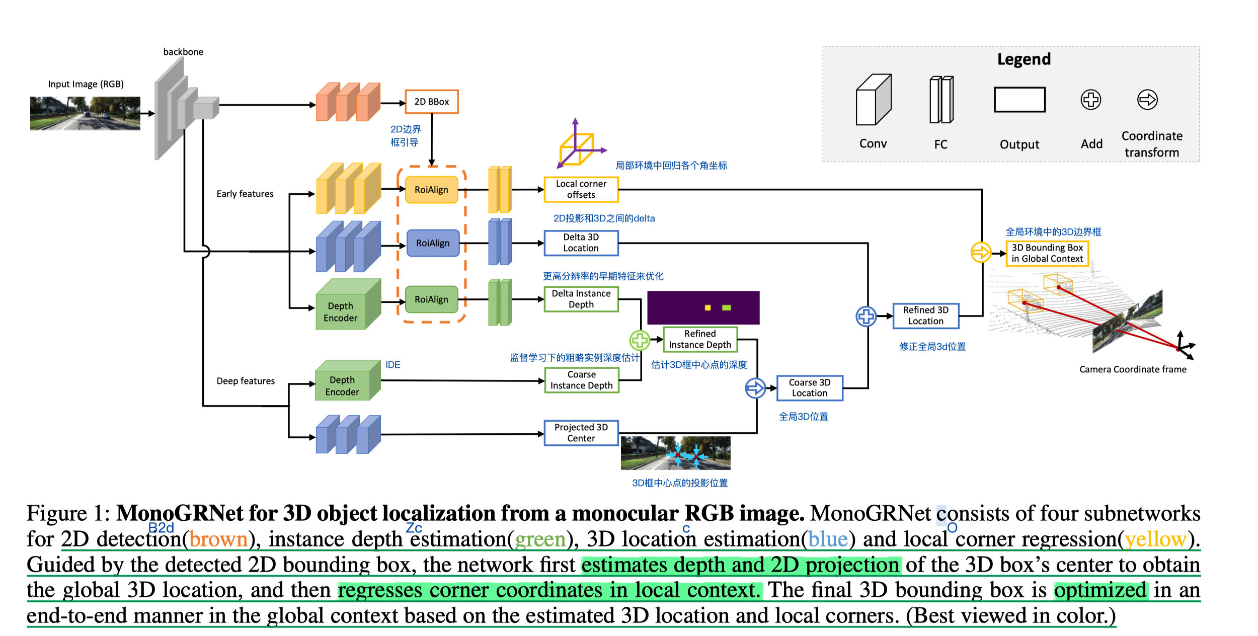
几个重点：

• 将 3D 定位问题解耦为几个渐进式子任务，分别为2D目标检测$B_{2d}$、实例级深度估计IDE$Z_c$、3D位置检测（2D中心点$c$包含$u,v$两个方向，3D中心点$C$包含$X,Y,Z$三个方向）、局部角落回归$\mathcal{O}$（公8个点）。每个子任务从单目 RGB 图像中学习，通过几何推断，在已观察到的二维投影平面和在未观察到的深度维度中定位物体非模态三维边界框（Amodal Bounding Box, ABBox-3D），即实现了由二维视频确定物体的三维位置。

  $$B_{3d} = (B_{2d}, Z_c, c, \mathcal{O})$$

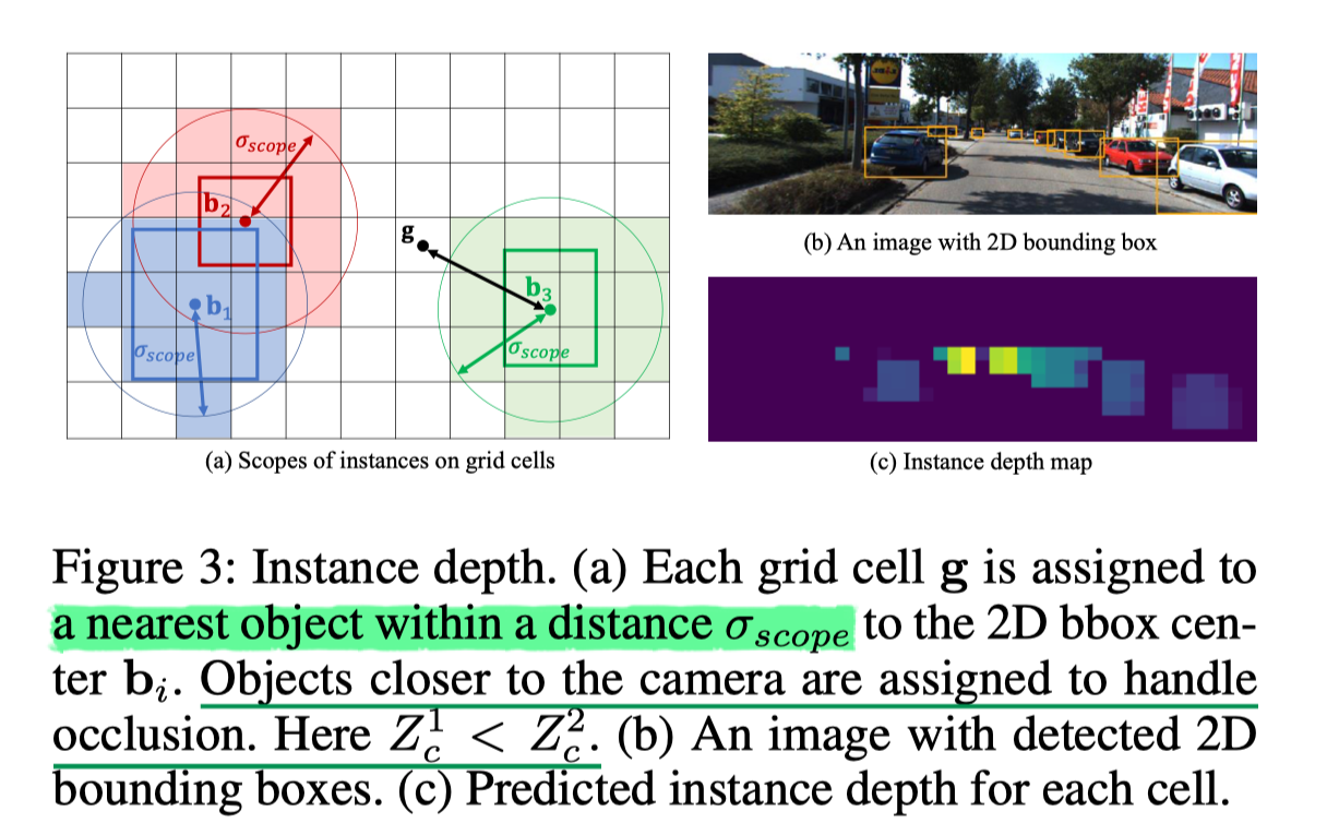
• 提出了instance depth estimation(IDE)，使用3D bounding box的中心点通过（稀疏地）监督来预测目标的深度，不需要考虑目标的规模以及2D的位置；之间的都是pixel-to-pixel，而在一张图片中，背景占大部分，因此我们用像素级别，并且通过平均误差来计算损失，实际上是不准确的；IDE模块探索深度特征映射的大型感知域以捕获粗略的实例深度，然后联合更高分辨率的早期特征 以优化 IDE。(可以看到深层网络提取的是粗略的全局信息，然后通过浅层的有细节的高分辨率的局部信息来修正，使得信息更加精确)，有点像centernet，通过中心回归。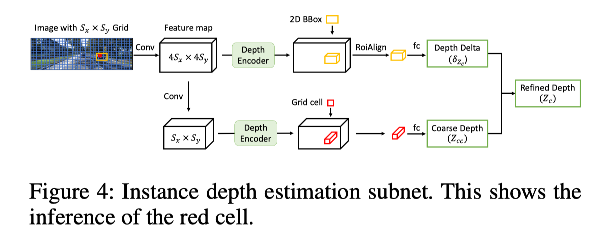

  

  $$Z_c = Z_{cc}+\delta_{Z_c}$$

• 全局3D位置，用公式将2D和3D的中心点进行转换（2D投影的中心点和3D的中心点不同），为了同时检索水平和垂直位置，首先要预测 3D 中心的 2D 投影。结合 IDE，然后将投影中心拉伸到真实 3D空间 以获得最终的3D对象位置。

  

  $$u=f_x*X/Z+p_x,\ v=f_y*Y/Z+p_y$$

  其中，$f_x, f_y$分别表示在X和Y轴上的焦距，$p_x,p_y$是坐标系的原点（coordinates of the principle point）

  这样在2D投影到3D的时候，就可以用：

  $$X=(u-p_x)*Z/f_x,\ Y=(v-p_y)*Z/f_y$$

  和IDE模块相似，我们使用early features来回归得到$\delta_C$，这样中心点的3D位置就可以用$C=C_s+\delta_C$。

• 局部角落回归，用高分辨率的信息来回归局部3D框的角点，根据图二的C图，从局部坐标到相机坐标的转换涉及到旋转$R$和平移$C$，全局角落坐标为$O_k^{cam}=RO_k+C$。

• 统一的网络结构，端到端训练，通过联合的几何损失函数进行优化，最大限度地减少 3D 边界在整体背景下的边界框的差异。

  • 2D检测（softmax[$s\cdot$] cross entropy[CE] loss + masked L1 distance[d] loss）：

    $$\mathcal L_{conf}=CE_{g\in\mathcal G}(s\cdot(Pr^g_{obj}),\tilde{Pr}^g_{obj})\\ \mathcal L_{bbox}=\sum_g\mathbb {1}_g^{obj}\cdot d(B_{2d}^g,\tilde B_{2d}^g)\\ \mathcal L_{2d} = \mathcal L_{conf} + \omega\mathcal L_{bbox}$$

    其中，Pr是置信度，$\mathbb 1_g^{obj}$是指示格子g中是否属于任何目标，如果格子g到最近的目标b的距离小于$\sigma_{scope}$，那么设置为1。

  • 实例深度预测（L1 loss）：

    $$\mathcal L_{zc}=\sum_g\mathbb {1}_g^{obj}\cdot d(Z_{cc}^g,\tilde Z_{c}^g)\\ \mathcal L_{z\delta}=\sum_g\mathbb {1}_g^{obj}\cdot d(Z_{cc}^g+\delta^g_{Z_c},\tilde Z_{c}^g)\\ \mathcal L_{depth} = \alpha\mathcal L_{zc} + \mathcal L_{z\delta}$$

    其中，$\alpha>1$，鼓励模型在粗略估计的时候已经接近真实值了。

  • 3D 定位损失（L1 loss）：

    $$\mathcal L_c^{2d}=\sum_g\mathbb {1}_g^{obj}\cdot d(g+\delta^g_{c},\tilde c{^g})\\ \mathcal L_{c}^{3d}=\sum_g\mathbb {1}_g^{obj}\cdot d(C_{s}^g+\delta^g_{C},\tilde C^g)\\ \mathcal L_{location} = \beta\mathcal L_{c}^{2d} + \mathcal L_{c}^{3d}$$

    其中，$\beta>1$，鼓励模型在学习投影中心点时已经接近真实值了。

  • 局部角点损失（L1 loss）：

    $$\mathcal L_{corners}=\sum_g\sum_k\mathbb 1^{obj}_g\cdot d(O_k,\tilde O_k)$$

  • 联合3D损失：

    $$\mathcal L_{joint}=\sum_g\sum_k\mathbb 1^{obj}_g\cdot d(O_k^{cam},\tilde O_k^{cam})$$

效果：在KITTI 数据集上，该网络在 3D 物体定位方面优于最先进的单目方法，且推理时间最短。

*Deep 3D box: 3d Bounding Box Estimation Using Deep Learning and Geometry——2017

这篇文章的特点在于提出的几何限制关系，以及提出了预测dimension这一stable属性。

In contrast to current techniques that only regress the 3D orientation of an object, our method first regresses relatively stable 3D object properties using a deep convolutional neural network and then combines these estimates with geometric constraints provided by a 2D object bounding box to produce a complete 3D bounding box. 之前的方法主要在意object的方向，但这篇文章增添了一些object的固定属性：choose to regress the box dimensions D rather than translation T because the variance of the dimension estimate is typically smaller (e.g. cars tend to be roughly the same size)。

同时利用了2D bbox和3D bbox之间的几何限制关系来限制9个DOF(three for translation, three for rotation, and three for box dimensions)。

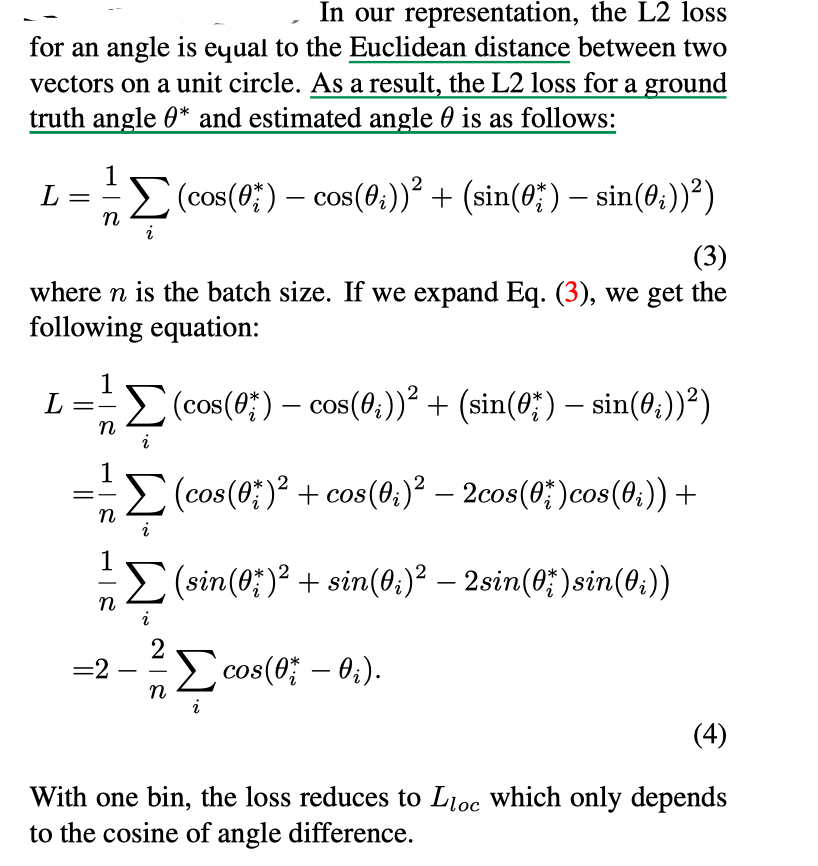
总体结构使用了MultiBin的思想，proposed MultiBin architecture for orientation estimation. We first discretize the orientation angle and divide it into n overlapping bins. For each bin, the CNN network estimates both a confidence probability $c_i$ that the output angle lies inside the $i^{th}$ bin and the residual rotation correction that needs to be applied to the orientation of the center ray of that bin in order to obtain the output angle. The residual rotation is represented by two numbers, for the sine and the cosine of the angle. Valid cosine and sine values are obtained by applying an L2 normalization layer on top of a 2-dimensional input. This results in 3 outputs for each bin $i:(c_i, \cos(\Delta \theta_i), sin(\Delta \theta_i))$.

def generate_bins(bins):
    angle_bins = np.zeros(bins)
    interval = 2 * np.pi / bins
    for i in range(1,bins):
        angle_bins[i] = i * interval
    angle_bins += interval / 2 # center of the bin

    return angle_bins

• The first network output estimates the 3D object orientation using a novel hybrid discrete-continuous loss, which significantly outperforms the L2 loss.
• The second output regresses the 3D object dimensions, which have relatively little variance compared to alternatives and can often be predicted for many object types. These estimates, combined with the geometric constraints (use the fact that the perspective projection of a 3D bounding box should fit tightly within its 2D detection window) on translation imposed by the 2D bounding box, enable us to recover a stable and accurate 3D object pose.

class Model(nn.Module):
      # ...
      def forward(self, x):
        x = self.features(x)  # 512 x 7 x 7
        x = x.view(-1, 512 * 7 * 7)
        orientation = self.orientation(x)
        orientation = orientation.view(-1, self.bins, 2)  # angle ssin + cos
        orientation = F.normalize(orientation, dim=2)
        confidence = self.confidence(x)
        dimension = self.dimension(x)
        return orientation, confidence, dimension

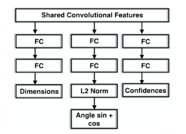
Loss for the MultiBin orientation is thus:

$$L_\theta = L_{conf} + w \times L_{loc}\\ L_{loc} = -\frac 1 {n_{\theta^*}}\sum cos(\theta^* − c_i − \Delta\theta_i )$$

def OrientationLoss(orient, angleDiff, confGT):
    #
    # orient = [sin(delta), cos(delta)] shape = [batch, bins, 2]
    # angleDiff = GT - center, shape = [batch, bins]
    #
    [batch, _, bins] = orient.size()
    cos_diff = torch.cos(angleDiff)
    sin_diff = torch.sin(angleDiff)
    cos_ori = orient[:, :, 0]
    sin_ori = orient[:, :, 1]
    mask1 = (confGT != 0)
    mask2 = (confGT == 0)
    count = torch.sum(mask1, dim=1)
    tmp = cos_diff * cos_ori + sin_diff * sin_ori
    tmp[mask2] = 0
    total = torch.sum(tmp, dim=1)
    count = count.type(torch.FloatTensor).cuda()
    total = total / count
    return -torch.sum(total) / batch
  
def OrientationLoss(orient_batch, orientGT_batch, confGT_batch):
    batch_size = orient_batch.size()[0]
    indexes = torch.max(confGT_batch, dim=1)[1]

    # extract just the important bin
    orientGT_batch = orientGT_batch[torch.arange(batch_size), indexes]
    orient_batch = orient_batch[torch.arange(batch_size), indexes]

    theta_diff = torch.atan2(orientGT_batch[:, 1], orientGT_batch[:, 0])
    estimated_theta_diff = torch.atan2(orient_batch[:, 1], orient_batch[:, 0])

    return -1 * torch.cos(theta_diff - estimated_theta_diff).mean()
  
def orientation_loss(y_true, y_pred):
    # Find number of anchors
    anchors = tf.reduce_sum(tf.square(y_true), axis=2)
    anchors = tf.greater(anchors, tf.constant(0.5))
    anchors = tf.reduce_sum(tf.cast(anchors, tf.float32), 1)

    # Define the loss
    loss = (y_true[:,:,0]*y_pred[:,:,0] + y_true[:,:,1]*y_pred[:,:,1])
    loss = tf.reduce_sum((2 - 2 * tf.reduce_mean(loss,axis=0))) / anchors

    return tf.reduce_mean(loss)

其中$L_{conf}$ is equal to the softmax loss of the confidences of each bin nn.CrossEntropyLoss(). $L_{loc}$ is the loss that tries to minimize the difference between the estimated angle and the ground truth angle in each of the bins that covers the ground truth angle, with adjacent bins having overlapping coverage.

由于下述关系，$L_{loc}$就只关联为cos部分。首先(gt_theta-pred_theta) 是在一个bins中与中心角的差值，所以在bins=2时，它的范围在[-pi/2, pi/2]，那么希望loss接近-1，即这一项趋向于0，即括号中的项应该是相同的；这里的theta是一个结果，output，而不是中间的值，所以根据导数反向传播修改的是内部参数，而因为内部参数变了，导致这次预测的theta是更靠近结果的

The loss for dimension estimation $L_{dims}$ is computed as follows(L2 loss nn.MSELoss()):

$$L_{dims}=\sum (D^∗− \bar D − \delta)^2 ,$$

几何限制关系：例如：$x_0=[d_x/2, -d_y/2, d_z/2]^T$的投影应该和2D框的最左边tightly。【同样对$x_{max},y_{min},y_{max}$也有类似的限制】

$$x_{min} = (k\left[\begin{matrix}R&T\end{matrix}\right]\left[\begin{matrix}d_x/2\\-d_y/2\\d_z/2\\1\end{matrix}\right])_x$$

Total loss is the weighted combination of

$$L = \alpha × L_{dims} + L_{\theta}$$

---

Introduce three additional performance metrics measuring the 3D box accuracy: distance to center of box, distance to the center of the closest bounding box face, and the over-all bounding box overlap with the ground truth box, measured using 3D Intersection over Union (3D IoU) score.

Mono3d：Monocular 3D Object Detection for Autonomous Driving——2016

主要思路就是利用3D包围框与2D包围框之间存在的映射联系，用2D空间中的特征来描述3D包围框。First aims to generate a set of candidate class-specific object proposals提出一种生成类相关的物体推荐候选框算法, which are then run through a standard CNN pipeline to obtain high-quality object detections.然后利用标准CNN来获得高质量的目标检测。The focus of this paper is on proposal generation. Propose an energy minimization approach that places object candidates in 3D using the fact that objects should be on the ground-plane利用物体和地平面接触的约束条件. We then score each candidate box projected to the image plane via several intuitive potentials encoding semantic segmentation, contextual information, size and location priors and typical object shape. 用SSVM对物体框打分，选取得分高的框进行分类和精细化的调整。

两个假设：

（三维空间离散化为立体像素边长为0.2m的三维模型）

1. 由于KITTI数据集的单目图像拍摄时相机在汽车上固定位置，因此地平面相对于相机的映射关系是固定的，同时作者假设所有图像的相机Y轴（也就是三维空间中的垂直方向）与地面是垂直的。
2. 所有的物体底部都与地平面相接。

• sample candidate bounding boxes with typical physical sizes in the 3D space by assuming a prior on the ground-plane. Represent each object with a 3D bounding box, y = (x, y, z, θ, c, t)(θ: azimuth angle, c: class, t: representative 3D templates)采样的时候认为不同类别的物体拥有不同的高度范围，这个范围误差在高斯函数的范围内。密集采样之后将内部像素完全是地面的物体框去除，同时去除具有非常低的3D位置先验概率的框。由于密集的采样（穷举），候选框使用积分图进行特征提取。

• project the boxes to the image plane, thus avoiding multi-scale search in the image

• score candidate boxes by exploiting multiple features: class semantic, instance semantic, contour, object shape, context, and location prior.

  scoring function:

  $$E(x, y) =w^T_{c,sem}\phi_{c,sem}(x, y) + w^T_{c,inst}\phi_{c,inst}(x, y)+ w^T_{c,cont}\phi_{c,cont}(x, y) + w^T_{c,loc}\phi_{c,loc}(x, y)+w^T_{c,shape}\phi_{c,shape}(x, y)$$

  • class semantic

    语义分割主要有两个衡量，一个是框内属于c的像素比例，另一个是框内不属于c的像素比例。

    Incorporate two types of features encoding semantic segmentation. The first feature encourages the presence of an object inside the bounding box by counting the percentage of pixels labeled as the relevant class:

    $$\phi_{c,seg}(x, y)=\frac{\sum_{i\in\Omega(y)}S_c(i)}{|\Omega(y)|}$$

    The second feature computes the fraction of pixels that belong to classes other than the object class:

    $$\phi_{c,non−seg,c'}(x, y)=\frac{\sum_{i\in\Omega(y)}S_c'(i)}{|\Omega(y)|}$$

  • instance semantic

    只对汽车进行实例分割

  • shape

    在2D的候选物体包围框中划分了两种栅格，其中，一种栅格图含有一个栅格，另一种栅格图含有K×K个栅格，统计这些栅格中每个栅格内的轮廓像素数量。

  • context

    用2D物体包围框的下方的1/3高度的区域作为上下文区域，用汽车下必然是地面这一上下文关系作为约束

  • location

    使用核密度估计(KDE)学习物体的位置先验信息，其中固定位置偏差为4m，2D图像位置偏差为两个像素

  Weight each loss equally, and define the category loss as cross entropy, the orientation loss as a smooth l1 and the bounding box offset loss as a smooth l1 loss over the 4 coordinates that parameterized the 2D bounding box.

• 利用CNN对高分框重新打分和分类，得到候选框的类别、精确位置以及方向信息

  

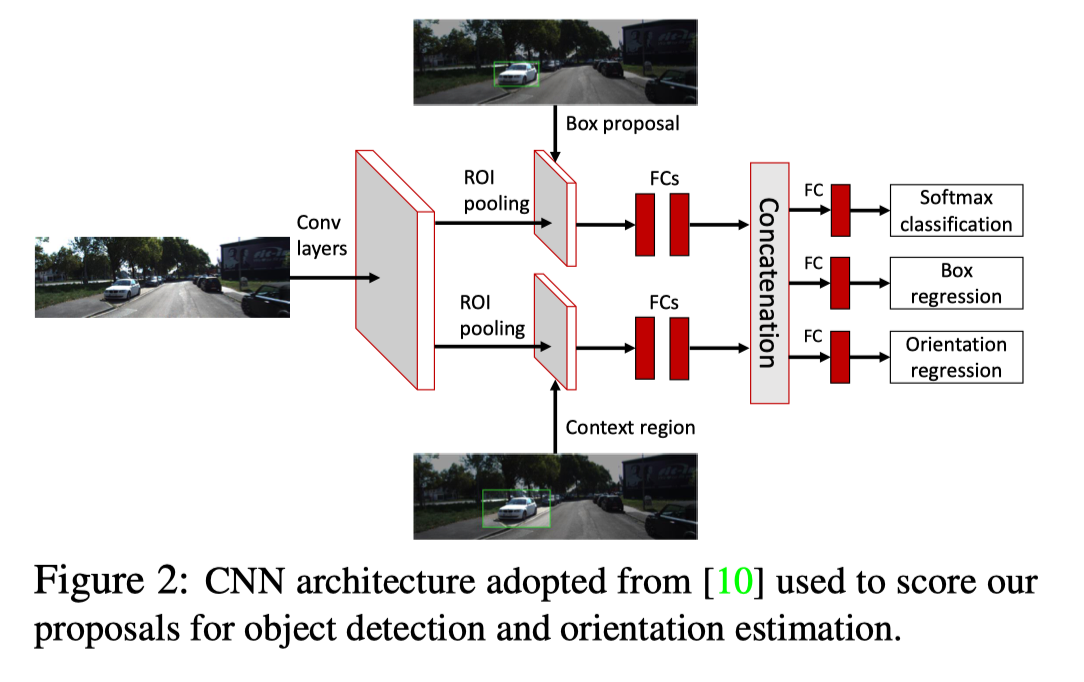
• A final set of object proposals is obtained after non-maximum suppression

RTM3D: Real-time Monocular 3D Detection from Object Keypoints for Autonomous Driving——2020

这一篇文章主要是将3D Detection问题转换为预测关键点问题；首先通过预测object的9个关键点（8个角点+1个中心点），然后通过几何关系（9个关键点，18个限制）得到dimension, location, and orientation。

整个网络由3个部分组成：backbone, keypoint feature pyramid, and detection head. 总体是one-stage的。

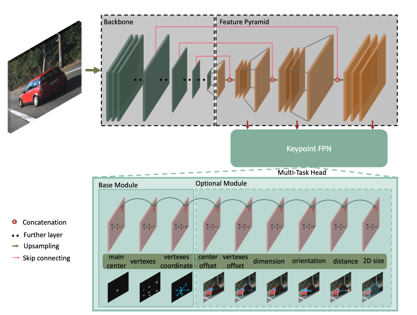
• backbone: ResNet-18 and DLA-34

• keypoint feature pyramid: Keypoint in the image have no difference in size. Therefore, the keypoint detection is not suitable for using the Feature Pyramid Network(FPN). Instead, propose Keypoint Feature Pyramid Network (KFPN) to detect scale-invariant key-points in the point-wise space.

  • F scale feature maps, first resize each scale f, back to the size of maximal scale, then yields the feature maps $f_{1<f<F}$
  • generate soft weight by a softmax operation to denote the importance of each scale
  • scale-space score map S score is obtained by linear weighing sum
  $$S_{score} = \sum_f \hat f\odot softmax(\hat f), \odot\text{:element-wise product}$$

• detection head

  • three fundamental components
    • Inspired by CenterNet, we take a keypoint as the main-center for connecting all features. The heatmap can be define as $M \in [0, 1]^{\frac H S \times \frac W S \times C}$ , where C is the number of object categories
    • heatmap of nine perspective points $V \in [0, 1]^{\frac H S \times \frac W S \times 9 }$ projected by vertexes and center of 3D bounding box
    • For keypoints association of one object, regress an local offset $V_c \in R^{\frac H S \times \frac W S \times 18}$ from the maincenter as an indication
  • six optional components
    • The center offset $M_{os} \in R^{\frac H S \times \frac W S \times 2}$ and vertexes offset $V_{os} \in R^{\frac H S \times \frac W S \times 2}$ are discretization error for each keypoint in heatmaps(这个和local offser有什么区别，一个是离main center点的offset，这个是从heatmap来看？)
    • The dimension $D \in R^{\frac H S \times \frac W S \times 3}$ of 3D object have a smaller variance, which makes it easy to predict.
    • The rotation $R(\theta)$ of an object only by parametrized by orientation $\theta (yaw)$. Multi-Bin based method to regress the local orientation. generates feature map of $O \in R ^{\frac H S \times \frac W S \times 8}$ orientation with two bins.2个bins4个值；加上confidence也是4个，总共8个。
    • regress $Z\in R^{\frac H S \times\frac W S \times1}$ the depth of 3D box center.

  获取bbox的：

  • main-center, center offset, wh

  获取3d corners：

  • Vertexes, vertexes offset, vertexes coordinate

  画图的时候未用到所以这些是在哪里起到限制作用的呢，（这些只是为了得到3D的信息）？：

  • orientation, dimension, depth

Loss:

• The all heatmaps of keypoint training strategy(focal loss)

  The loss solves the imbalance of positive and negative samples with focal loss.

  

  K is the channels of different keypoints, K = C in maincenter and K = 9 in vertexes. N is the number of maincenter or vertexes in an image, and $\alpha$ and $\beta$ are the hyper-parameters to reduce the loss weight of negative and easy positive samples. We set is $\alpha = 2$ and $\beta = 4$. $p_{kxy}$ can be defined by Gaussian kernel $p_{xy} = exp(-\frac{x^2+y^2}{2\sigma})$ centered by ground truth keypoint $\tilde p_{xy}$. For $\sigma$, we find the max area $A_{max}$ and min area $A_{min}$ of 2D box in training data and set two hyperparameters $\sigma_{max}$ and $\sigma_{min}$. We then define the $\sigma = A( \frac{\sigma_{max} - \sigma_{min}}{A_{max} - A_{min}})$ for a object with size A.

• Regression of dimension and distance(residual term)

  

  $$\Delta \tilde D_{xy}=\log \frac{\tilde D_{xy}-\bar D}{D_{\sigma}}$$ $$1^{obj}_{xy}\text{ if maincenter appears in position x, y.}$$

• offset of maincenter, vertexes(L1)

  

• coordinate of vertexes(L1)

  

• All(multi-task)

  

Our goal is to estimate the 3D bounding box, whose projections of center and 3D vertexes on the image space best fit the corresponding 2D keypoint. We formulate it and other prior errors as a nonlinear least squares optimization problem:

由特征点检测网络给出9个特征 $\widehat{k p}_{i j}$ 点、物体尺寸 $D_{i} 、$ 方向 $\hat{\theta}_{i}$ 和中心点深度 $\widehat{Z}_{i}$ 后, $3 \mathrm{D}$ BBox就容易求了，如下式所示。 $R^{}, T^{}, D^{*}=\underset{\{R, T, D\}}{\arg \min } \sum_{R_{i}, T_{i}, D_{i}}\left|e_{c p}\left(R_{i}, T_{i}, D_{i}, \widehat{k p}_{i}\right)\right|_{\Sigma_{i}}^{2}+\omega_{d}\left|e_{d}\left(D_{i}, \widehat{D}_{i}\right)\right|_{2}^{2}+\omega_{r}\left|e_{r}\left(R_{i}, \hat{\theta}_{i}\right)\right|_{2}^{2}$
其中 $e_{c p}$ 是3D BBox的八个顶点和中心点到 $\widehat{k p}_{i j}$ 的重投影误差。八个顶点和中心点可以通过 $R, T, D$ 得到。 $\quad \Sigma_{i}=\operatorname{diag}\left(\operatorname{softmax}\left(V\left(\widehat{k p}_{i}\right)\right)\right.$ 为特征点检测的置信度，这里可以衡量各误差

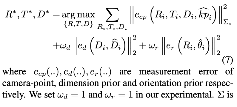
the covariance matrix of keypoints projection error.

一些error的计算，SE3 space: special euclidian 3-space.

Evaluation:

• Average precision for 3D intersection-over-union (AP 3D)
• Average precision for Birds Eye View (AP BEV )
• Average Orientation Similarity (AOS) if 2D bounding box available.

非官方复现上，对于depth使用了sigmoid，应该是为了平滑吧

一个问题就是得到这么多信息后，但是复原image并没有都用上，那为什么需要预测呢？感觉复原image的那部分预测的是在camera坐标系下的，后面是实际3D，但这样就不算3D了

IDA-3D: Instance-Depth-Aware 3D Object Detection from Stereo Vision for Autonomous Driving

stereo images, not rely on depth, A stereo RPN module is introduced to produce a pair of union RoI to avoid complex matching of the same object in a left-right image pair(关注instance not pixel) and reduce the interference of background on depth estimation. Pays more attention on far-away objects by disparity adaptation and matching cost reweighting. 这篇文章主要就是用instance简化了pixel，然后用了概率去选择一个depth level（其实也是个multibin的思想），同时根据disparity和depth的关系，修正了转换关系，最后加上了左右图之间关系连接的一个weight

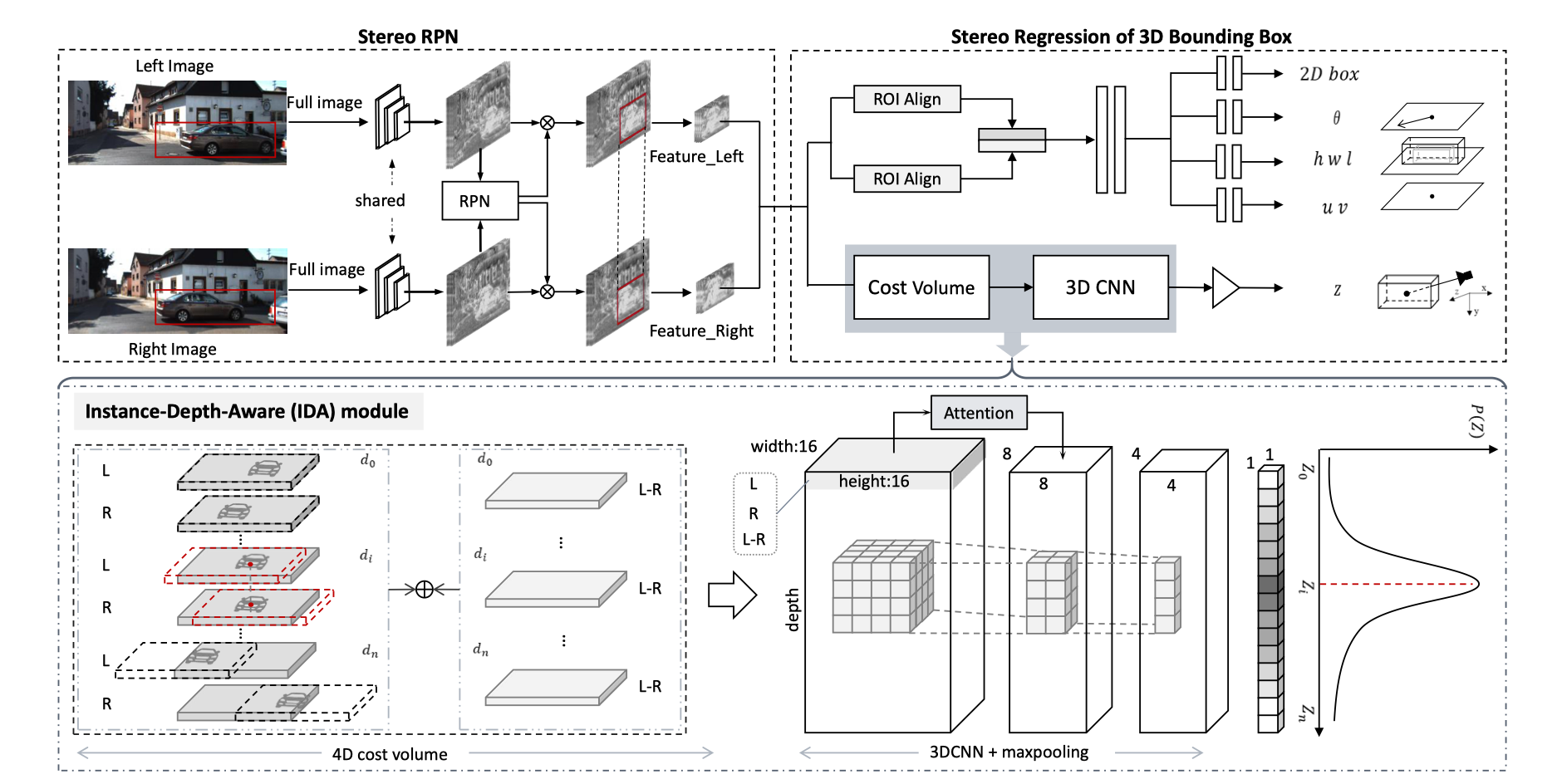
• design a six-parallel fully-connected network?(5个+1个RPN？)

  • 角度multibins
  • 维度，预测$\Delta$，然后用平均值与e的$\Delta$次方的乘积作为实际值
  • Multi-task loss

• computing the disparity of each instance to locate its position.disparity×height×width×feature size

  • employ two consecutive 3D convolution layers, each followed by a 3D max-pooling layer

  • 监督学习预object中心点的depth；N个depth level（实验中分了24个）, 给出每一个可能性，最后预测的depth

    $$\hat z=\sum_{i=0}^N z_iP(i)$$

    然后和gt进行smooth L1损失计算

• 修正depth：for the same disparity error, the error in depth increases quadratically with distance. It means that the influence of the disparity error in depth estimation of a far-away object is greater than a nearby one.如下图所示

  

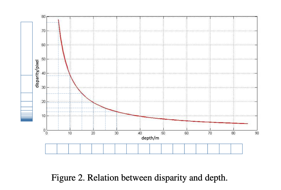
  • In order to adapt the model and loss function to lay more emphasis on a far-away object, we change the disparity level in cost volume from uniform quantization to nonuniform quantization where the farther the object is, the less the partition cell between two consecutive disparity levels.转换公式：

    $$D=\frac {f_u\times b}{z}$$

    $f_u$: horizontal focal length, b: baseline of binocular camera

    我们不必估算0-80m范围内的深度，因为汽车的深度与图像中的尺寸成反比?Given camera intrinsic parameters, we can roughly calculate the range according to the width of the union box in the image.只评估在一定范围内的

• Cost weighting

  To penalize the depth levels that are not unique for an object instance and promote the depth levels that have high prob-abilities, we reweight the matching cost.

  The first part in 4D volume packing a difference feature map between the left and right feature maps across each disparity level（in a certain depth level and refine depth estimation） and second part in 3DCNN employing attention mechanism on depth（sets the weight $r_i$ for each channel）. The correlation score $r_i$ that is obtained by calculating the correlation between left and right feature maps on each disparity is defined as: 就是左右两边特征图求cos相似性

  $$r_i = cos<F^l_i,F^r_i>=\frac{F^l_i\cdot F^r_i}{\|F^l_i\|\cdot \|F^r_i\|}$$

SMOKE: Single-Stage Monocular 3D Object Detection via Keypoint Estimation——2020

old: In case of monocular vision, successful methods have been mainly based on two ingredients: (i) a network generating 2D region proposals, (ii) a R-CNN structure predicting 3D object pose by utilizing the acquired regions of interest.

This: predicts a 3D bounding box for each detected object by combining a single keypoint estimate with regressed 3D variables. As a second contribution, we propose a multi-step disentangling approach for constructing the 3D bounding box, which significantly improves both training convergence and detection accuracy. In contrast to previous 3D detection techniques, our method does not require complicated pre/post-processing, extra data, and a refinement stage. 总结来说就是包含关键点预测和3D变量回归两个模块的一阶段单目3D检测方法。

---

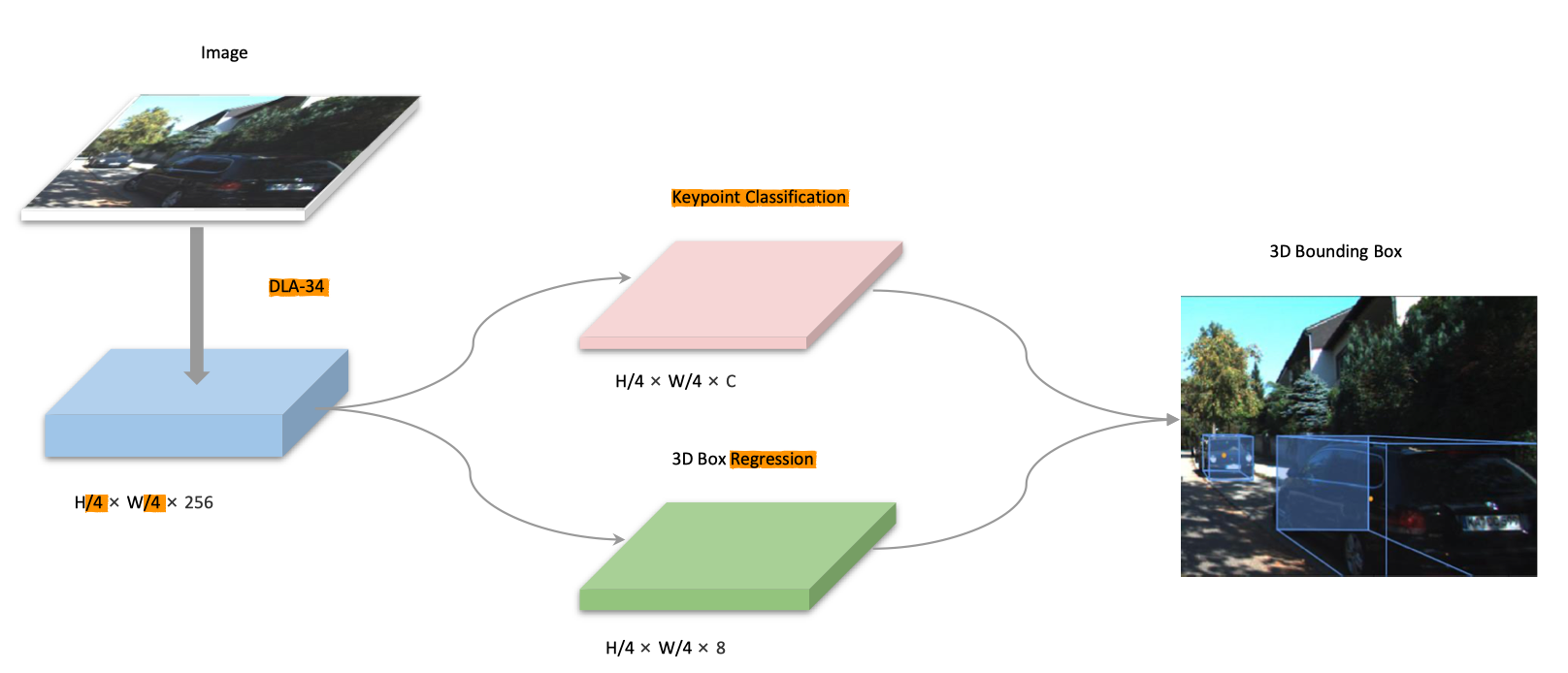
• Problem: A single RGB image $I \in R^{W\times H\times3}$ , find for each present object its category label C and its 3D bounding box B, where the latter is parameterized by 7 variables $(h, w, l, x, y, z, θ)$. ($(x, y, z)$ is the coordinates (in meters) of the object center in the camera coordinate frame.)

• Backbone: DLA-34 since it can aggregate information across different layers.

  • all the hierarchical aggregation connections are replaced by a Deformable Convolution Network (DCN).

  • The output feature map is downsampled 4 times with respect to the original image.

  • Replace all BatchNorm (BN) operation with GroupNorm (GN), since less sensitive to batch size and more robust to training noise

    • BN以batch的维度做归一化，依赖batch，过小的batch size会导致其性能下降，如果太大，显存又可能不够用，一般来说每GPU上batch设为32最合适。但这个维度并不是固定不变的，比如训练和测试时一般不一样，一般都是训练的时候在训练集上通过滑动平均预先计算好平均-mean，和方差-variance参数。而在测试的时候，不再计算这些值，而是直接调用这些预计算好的来用，但当训练数据和测试数据分布有差别时，训练时上预计算好的数据并不能代表测试数据，这就导致在训练，验证，测试这三个阶段存在不一致。

    • GN：同样可以解决Internal Covariate Shift的问题，channel方向每个group的均值和方差

      def GroupNorm(x, gamma, beta, G, eps=1e-5):
          # x: input features with shape [N,C,H,W]
          # gamma, beta: scale and offset, with shape [1,C,1,1]
          # G: number of groups for GN
          N, C, H, W = x.shape
          x = tf.reshape(x, [N, G, C // G, H, W])
          mean, var = tf.nn.moments(x, [2, 3, 4], keep dims=True)
          x = (x - mean) / tf.sqrt(var + eps)
          x = tf.reshape(x, [N, C, H, W])
          return x * gamma + beta

    BatchNorm：batch方向做归一化，算$N*H*W$的均值
    LayerNorm：channel方向做归一化，算$C*H*W$的均值
    InstanceNorm：一个channel内做归一化，算$H*W$的均值
    GroupNorm：将channel方向分group，然后每个group内做归一化，算$(C//G)*H*W$的均值

    GN比LN效果好的原因是GN比LN的限制更少，因为LN假设了一个层的所有通道的数据共享一个均值和方差。而IN则丢失了探索通道之间依赖性的能力。

    

• 3D Detection Network

  • Keypoint Branch: the key point is defined as the projected 3D center of the object on the image plane.

    $$\left[\begin{matrix}x&y&z\end{matrix}\right]^T$$ represent the 3D center of each object in the camera frame. The projection of 3D points to points  $$\left[\begin{matrix}x_c&y_c\end{matrix}\right]^T$$on the image plane can be obtained with the camera intrinsic matrix K in a homogeneous form:$$

    \left[\begin{matrix}z\cdot x\\z\cdot y\\z\end{matrix}\right]=K_{3\times 3}\left[\begin{matrix}x\\y\\z\end{matrix}\right]
    $$
    Downsampled location on the feature map is computed and distributed using a Gaussian Kernel.

    

  • Regression Branch: the 3D information is encoded as an 8-tuple $\tau =\left[\begin{matrix}\delta_z&\delta_{x_c}&\delta_{y_c}&\delta_h&\delta_w&\delta_l&\sin\alpha&\cos \alpha\end{matrix}\right]^T$ . $\delta_{x_c} , \delta_{y_c}$ is the discretization offset due to downsampling, $\delta_h,\delta_w,\delta_l$ denotes the residual dimensions. We encode all variables to be learnt in residual representation to reduce the learning interval and ease the training task. A similar operation F that converts projected 3D points to a 3D bounding box $B = F(\tau) \in \mathbb R^{3\times 8}$ .

    • For each object, its depth z can be recovered by predefined scale and shift parameters $\sigma_z, \mu_z$ as

      $$z=\mu_z+\delta_z\sigma_z$$

      这样上述的the location for each object in the camera frame可以表示为：

      $$\left[\begin{matrix}x\\y\\z\end{matrix}\right]=K_{3\times 3}^{-1}\left[\begin{matrix}z\cdot (x_c+\delta_{x_c})\\z\cdot (y_c+\delta_{y_c})\\z\end{matrix}\right]$$

      对于dimensions的部分，使用每一个类别预先设定好的平均值（从整个数据集中先计算平均值）pre-calculated category-wise average dimension作为一个base，然后用residual representation来计算出真实的维度。

      $$\left[\begin{matrix}h\\w\\l\end{matrix}\right]=\left[\begin{matrix}\bar h\cdot e^{\delta_h}\\\bar w\cdot e^{\delta_w}\\\bar l\cdot e^{\delta_l}\end{matrix}\right]$$

      对于角度部分，Regress the observation angle $\alpha$ instead of the yaw rotation $\theta$ for each object. [from. “3D bounding box estimation using deep learning and geometry”]. We further change the observation angle with respect to the object head $\alpha_x$ , instead of the commonly used observation angle value $\alpha_z$ , by simply adding $\frac \pi 2$ .

      

      因此最终预测的yaw：

      $$\theta = \alpha_z + arctan(\frac{x}{z})$$

      Bounding box：

      $$B=R_{\theta}\left[\begin{matrix}\pm h/2\\\pm w/2\\\pm l/2\end{matrix}\right]+\left[\begin{matrix}x\\y\\z\end{matrix}\right]$$

• Loss

  • Keypoint Classification Loss

    Penalty-reduced focal loss in a point-wise. $s_{i,j}$ be the predicted score at the heatmap location $(i, j)$ and $y_{i,j}$ be the ground-truth value of each point assigned by Gaussian Kernel.

    定义$\breve y_{i,j},\breve s_{i,j}$：

    $$\breve y_{i,j}=\begin{cases}0,\ if\ y_{i,j}=1\\y_{i,j},\ otherwise \end{cases}\\ \breve s_{i,j}=\begin{cases}s_{i,j},\ if\ y_{i,j}=1\\1-s_{i,j},\ otherwise \end{cases}$$

    简化为同一个类别，则分类损失函数：

    $$L_{cls}=-\frac 1 N\sum_{i,j=1}^{h,w}(1-\breve y_{i,j})^{\beta}(1-\breve s_{i,j})^{\alpha}\log(\breve s_{i,j})$$

    N是图片中object的数量，即$y_{i,j}=1$的个数；The term $(1 − y_{i,j} )$ corresponds to penalty reduction for points around the groundtruth location. 从整个损失函数来看，中心点希望score尽可能的大，远离部分的点，希望score尽可能的小

  • Regression Loss（observe that l1 loss performs better than Smooth l1 loss）

    add channel-wise activation to the regressed parameters of dimension and orientation at each feature map location to preserve consistency. The activation functions for the dimension and the orientation are chosen to be the sigmoid function $\sigma$ and the $l2$ norm, respectively:

    $$\left[\begin{matrix}\delta_h\\\delta_w\\\delta_l\end{matrix}\right]=\sigma\left(\begin{matrix}o_h\\o_w\\o_l\end{matrix}\right)-\frac 1 2\\ \left[\begin{matrix}\sin \alpha\\\cos \alpha\end{matrix}\right]=\left[\begin{matrix}o_{\sin}/\sqrt{o_{sin}^2+o^2_{cos}}\\o_{\cos} /\sqrt{o_{sin}^2+o^2_{cos}}\end{matrix}\right]$$

    o stands for the specific output of network. The 3D bounding box regression loss as the l1 distance between pred and gt. λ is a scaling factor.

    $$L_{reg}=\frac \lambda N\|\hat B-B\|_1$$

  • The final loss function(three different groups: orientation, dimension and location.)

    $$L = L_{cls} + \sum_{i=1}^3 L_{reg}(\hat B_i)$$

---

细节处理：

• 数据处理：去除3D中心点在图像外侧的框

• 数据增强：random horizontal flip, random scale(9 steps from 0.6 to 1.4) and shift(5 steps from -0.2 to 0.2). Note that the scale and shift augmentation methods are only used for heatmap classification since the 3D information becomes inconsistent with data augmentation. 应该是指数据增强部分只是为了hm分类，并不作用到3D检测上；从代码来看，增加了一个flag，相当于最后预测完之后，再逆方向返回，得到未增强后的3D信息

• 超参数：In the backbone, the group number for GroupNorm is set to 32. For channels less than 32, it is set to be 16. Set $\alpha = 2, \beta = 4, \left[\begin{matrix}\bar h& \bar w&\bar l\end{matrix}\right]^T =\left[\begin{matrix}1.63&1.53&3.88\end{matrix}\right]^T, \left[\begin{matrix}\mu_z&\sigma_z\end{matrix}\right]^T=\left[\begin{matrix}28.01&16.32\end{matrix}\right]^T$.

• 训练：use the original image resolution and pad it to 1280 × 384. The learning rate is set at $2.5 × 10^{−4}$ and drops at 25 and 40 epochs by a factor of 10.

• 测试：Use the top 100 detected 3D projected points and filter it with a threshold of

  0.25. No data augmentation method and NMS are used in the test procedure.

Shift R-CNN

第1阶段：faster R-CNN，增加3D角度和尺寸回归。 第2阶段：用相机投影几何约束进行3D平移的闭式解方案。第3阶段：ShiftNet细化和最终3D目标框重建。

GS3D

大范围的回归通常不比离散分类好，因此将残差回归转换为3D边框细化的分类过程。其主要思想是将残差范围划分为多个区间，识别残差值是位于其中一个区间。

OFT: Orthographic Feature Transform for Monocular 3D Object Detection——2018

One explanation for this performance gap(lidar-based with image-based) is that existing systems are entirely at the mercy of the perspective image-based representation, in which the appearance and scale of objects varies drastically with depth and meaningful distances are difficult to infer.

Escape the image domain by mapping image-based features into an orthographic 3D space.

---

five main components:

• Front-end ResNet without bottleneck layers: feature extractor, a hierarchy of multi-scale, aim to eliminate variance to scale

• Orthographic feature transform: a differentiable transformation which maps a set of features extracted from a perspective RGB image to an orthographic birds-eye-view feature map.

  

  • 3D voxel feature map $g(x,y,z)\in \mathbb R^n$ with relevant n-dimensional features from the image-based feature map $f(u,v)\in \mathbb R^n$. The voxel map is defined over a uniformly spaced 3D lattice $\mathcal G$. fixed to the ground plane a distance y0 below the camera and has dimensions W, H, D and a voxel size of r.

    • approximate r by a rectangular bounding box

      $$\begin{aligned} &u_{1}=f \frac{x-0.5 r}{z+0.5 \frac{x}{|x|} r}+c_{u}, \quad v_{1}=f \frac{y-0.5 r}{z+0.5 \frac{y}{|y|} r}+c_{v}\\ &u_{2}=f \frac{x+0.5 r}{z-0.5 \frac{x}{|x|} r}+c_{u}, \quad v_{2}=f \frac{y+0.5 r}{z-0.5 \frac{y}{|y|} r}+c_{v} \end{aligned}$$

      f: camera focal length c: principle point

    • appropriate location in the voxel feature map g by average pooling over the projected voxel’s bounding box in the image feature map f

      $$\mathbf{g}(x, y, z)=\frac{1}{\left(u_{2}-u_{1}\right)\left(v_{2}-v_{1}\right)} \sum_{u=u_{1}}^{u_{2}} \sum_{v=v_{1}}^{v_{2}} \mathbf{f}(u, v)$$

    • But this is extremely memory intensive.

  • applications such as autonomous driving where most objects are fixed to the 2D ground plane, we can make the problem more tractable by collapsing the 3D voxel feature map down to a third, two-dimensional representation which we term the orthographic feature map h(x, z).

    • The orthographic feature map is obtained by summing voxel features along the vertical axis after multiplication with a set of learned weight matrices.

      $$\mathbf{h}(x, z)=\sum_{y=y_{0}}^{y_{0}+H} W(y) \mathbf{g}(x, y, z)$$

    • A major challenge with the above approach is the need to aggregate features over a very large number of regions.

  • integral feature map, F, is constructed from an input feature map f using the recursive relation

    $$F(u,v)=f(u,v)+F(u-1, v)+F(u, v-1)-F(u-1, v-1)$$

    Then

    $$g(x,y,z)=\frac{F(u_1,v_1)+F(u_2,v_2)-F(u_1,v_2)-F(u_2,v_1)}{(u_2-u_1)(v_2-v_1)}$$

• Topdown network: consisting of a series of ResNet residual units, processes the BEV feature maps in a manner which is invariant to the perspective effects observed in the image. Emphasize the importance of reasoning in 3D for object recognition and detection in complex 3D scenes.

  • ResNet-style skip connections

• Output heads

  • Confidence map, S(x, z) is a smooth Gaussian function. l1 loss.

    $$S(x, z)=\max _{i} \exp \left(-\frac{\left(x_{i}-x\right)^{2}+\left(z_{i}-z\right)^{2}}{2 \sigma^{2}}\right)$$

    vastly fewer positive (high confidence) locations than negative ones, which leads to the negative component of the loss dominating optimization. It is coarse approximation. To overcome this we scale the loss corresponding to negative locations (which we define as those with S(x, z) < 0.05) by a constant factor of 10 −2 .

  • as a classification problem, with a cross entropy loss.

  • Localization and bounding box estimation. In order to localize each object more precisely, l1 loss.

    $$\boldsymbol{\Delta}_{\boldsymbol{p o s}}(x, z)=\left[\frac{x_{i}-x}{\sigma} \quad \frac{y_{i}-y_{0}}{\sigma} \quad \frac{z_{i}-z}{\sigma}\right]^{\top}$$

  • the dimension head, predicts the logarithmic scale offset. l1 loss.

    $$\boldsymbol{\Delta}_{\text {dim }}(x, z)=\left[\log \frac{w_{i}}{\bar{w}} \quad \log \frac{h_{i}}{h} \quad \log \frac{l_{i}}{l}\right]^T$$

  • the orientation head, predicts the sine and cosine. l1 loss.

    $$\boldsymbol{\Delta}_{\text {ang }}(x, z)=\left[\sin \theta_i \quad \cos\theta_i\right]^T$$

• Non-maximum suppression and decoding stage(peaks in the confidence maps and discrete bounding box predictions)

  use of confidence maps in place of anchor box classification is that we can apply NMS in the more conventional image processing sense

M3D-RPN

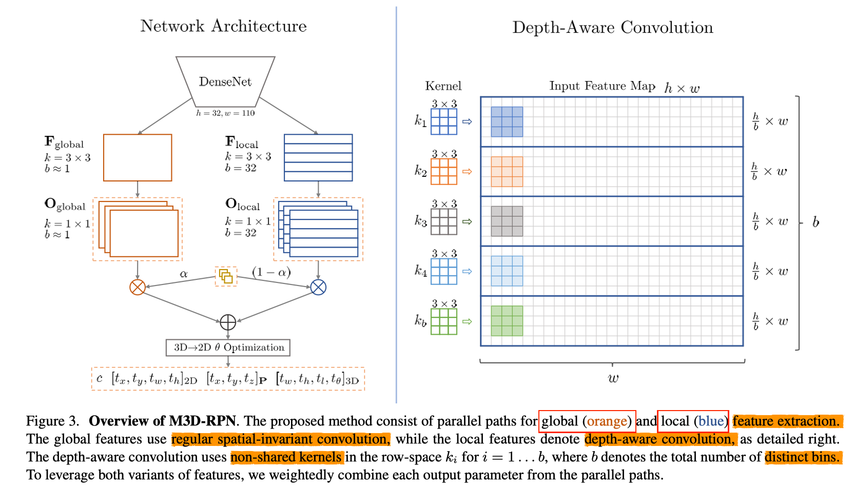
Propose to reduce the gap by reformulating the monocular 3D detection problem as a standalone 3D region proposal network. Design depth-aware convolutional layers which enable location specific feature development and in consequence improved 3D scene understanding.

---

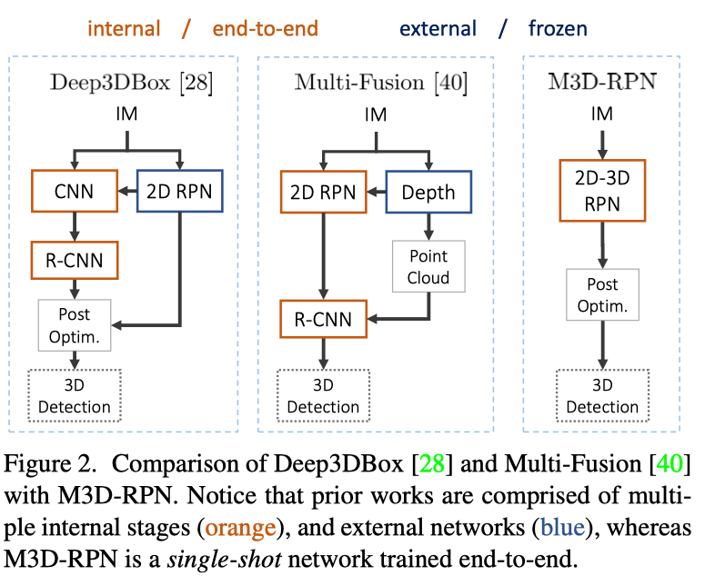
Contributions:

• Formulate a standalone monocular 3D region proposal network (M3D-RPN) with a shared 2D and 3D detection space, while using prior statistics to serve as strong initialization for each 3D parameter. 将各个参数初始化为先验值，可以使得每一个独立的anchor有强大的3D先验知识。同时生成2D和3D的proposals

  • Anchor

    首先2D和3D是共享参数——中心点位置$[x,y]_P$的，来一起寻找proposal，即之后去求出$[w,h]_{2D},z_P, [w,h,l,\theta]_{3D}$。那么对于2Dbbox其实已经可以确定了，对于3D的框，用$[x,y,z]_P$可以得到空间中的中心点坐标，然后根据剩下4个信息就可以得到3D世界下的anchor了。这里的P是增加了一维[0,0,0,1].

    $$\left[\begin{matrix}x\cdot z\\y\cdot z\\z\end{matrix}\right]_P=P\cdot\left[\begin{matrix}x\\y\\z\\1\end{matrix}\right]_{3D}$$

    The outputs of $[t_x , t_y , t_w , t_h ]_{2D}$ represent the 2D bounding box transformation.

    $$x'_{2D}=x_P+t_{x_{2D}}\cdot w_{2D}, \ y'_{2D}=y_P+t_{y_{2D}}\cdot h_{2D}, \\ w'_{2D}=exp(t_{w_{2D}})\cdot w_{2D}, \ h'_{2D}=exp(t_{h_{2D}})\cdot h_{2D}$$

    3D outputs:

    $$x'_{P}=x_P+t_{x_{P}}\cdot w_{2D}, \ y'_{P}=y_P+t_{y_{P}}\cdot h_{2D}, \ z'_{P}=t_{z_{P}}\cdot z_{P}\\ w'_{3D}=exp(t_{w_{3D}})\cdot w_{3D}, \ h'_{3D}=exp(t_{h_{3D}})\cdot h_{3D}, \ l'_{3D}=exp(t_{l_{3D}})\cdot l_{3D}\\ \theta'_{3D}=t_{\theta_{3D}}\cdot \theta_{3D}$$

  • Loss

    $$L=L_c+\lambda_1L_{b_{2D}}+\lambda_2L_{b_{3D}}\\ L_c=-\log(\frac{exp(c_\tau)}{\sum_i^{n_c}exp(c_i)})\\ L_{b_{2D}}=-\log(IoU(b'_{2D},\hat b_{2D}))\\ L_{b_{3D}}=SmoothL_1(b_{3D},\hat g_{3D})$$

• Propose depth-aware convolution to improve the 3D parameter estimation, thereby enabling the network to learn more spatially-aware high-level features. high-level features improve when given increased awareness of their depth and while assuming a consistent camera scene geometry.

  • Drawback: increase of memory footprint for a given layer by ×b.
  • connect two parallel paths at the end of the backbone network.
    • uses regular convolution where kernels are shared spatially, which we refer to as global.
    • The second path exclusively uses depth-aware convolution and is referred to as local.

• Propose a simple orientation estimation post-optimization algorithm which uses 3D → 2D projection consistency loss within a post-optimization algorithm.

  • using a learned attention $\alpha$. $$O^i=O^i_{global}\cdot\alpha_i+O^i_{local}\cdot(1-\alpha_i)$$

  

  

---

generate_anchors()
compute_bbox_stats()
init_training_model()
for iteration in range(start_iter, conf.max_iter):
  iterator, images, imobjs = next_iteration()
  adjust_lr()
  cls, prob, bbox_2d, bbox_3d, feat_size = M3D_rpn_net()
  det_loss, det_stats = criterion_det(cls, prob, bbox_2d, bbox_3d, imobjs, feat_size)
  if total_loss > 0:
			total_loss.backward()
  compute_stats(tracker, stats)

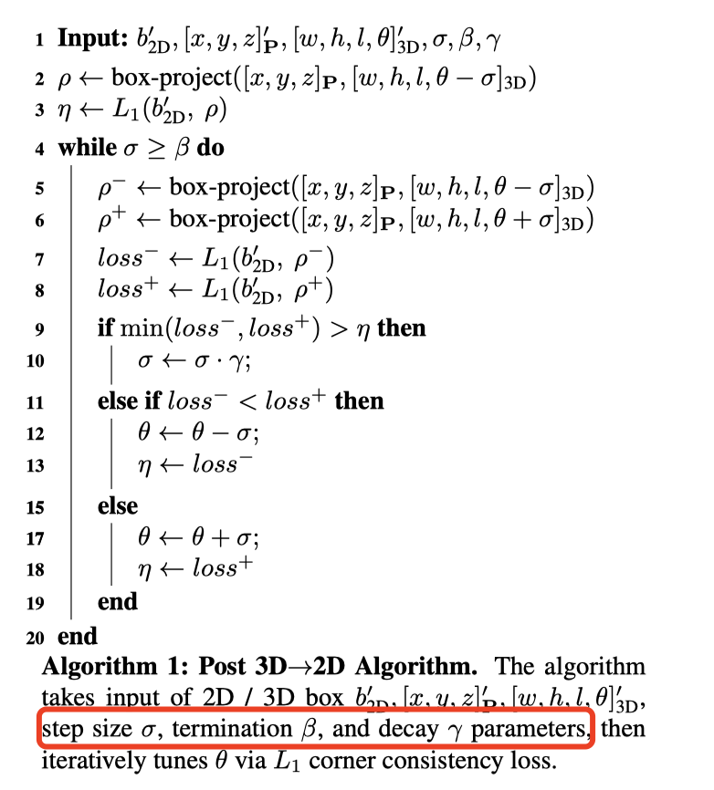
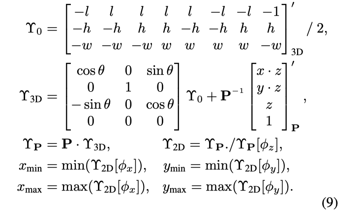
MonoPSR

Pseudo-LiDAR

3D-Deepbox

Joint Monocular 3D Vehicle Detection and Tracking——2019

An online network architecture to jointly track and detect vehicles in 3D from a series of monocular images.The framework can not only associate detections of vehicles in motion over time, but also estimate their complete 3D bounding box information from a sequence of 2D images captured on a moving platform. Design a motion learning module based on an LSTM for more accurate long-term motion extrapolation. Robust tracking helps 3D detection. leverage novel occlusion-aware association and depth-ordering matching algorithms to overcome the occlusion and reappearance problems in tracking. Update their 3D poses using LSTM motion estimation along a trajectory, integrating single-frame observations associated with the instance over time.

---

检测state：

$$s_a=(P,O,D,F,\Delta P)$$

P代表position,$(x,y,z)$；$\Delta P$代表速度, $(\dot{x}, \dot{y}, \dot{z})$, O朝向角，D维度$(l,w,h)$，F代表appearance feature。M(X)表示投影的2D外围框。

Assocation and Tracking

通过前后帧同一object应该有部分重叠，并且相似性高这一特点。

$$\begin{array}{c} \mathbf{A}_{\mathrm{deep}}\left(\tau_{a}, \mathbf{s}_{a}\right)=\exp \left(-\left\|F_{\tau_{a}}, F_{\mathbf{s}_{a}}\right\|_{1}\right) \\ \mathbf{A}_{2 \mathrm{D}}\left(\tau_{a}, \mathbf{s}_{a}\right)=\frac{\mathbf{d}_{\tau_{a}} \cap \mathbf{d}_{\mathbf{s}_{a}}}{\mathbf{d}_{\tau_{a}} \cup \mathbf{d}_{a}} \\ \mathbf{A}_{3 \mathrm{D}}\left(\tau_{a}, \mathbf{s}_{a}\right)=\mathbb{1} \times \frac{\phi\left(\mathbf{M}\left(X_{\tau_{a}}\right)\right) \cap \mathbf{M}\left(X_{\mathbf{s}_{a}}\right)}{\phi\left(\mathbf{M}\left(X_{\tau_{a}}\right)\right) \cup \mathbf{M}\left(X_{\mathbf{s}_{a}}\right)}\\ \left.\phi(\cdot)=\underset{x}{\arg \min }\left\{ x \mid \text { ord }(x)<\text { ord }\left(x_{0}\right) \forall x_{0} \in \mathbf{M}\left(X_{\tau_{a}}\right)\right)\right\} \end{array}$$

其中A是affinity matrix，第一个参数表示存在的tracking序列，第二个参数表示候选的状态，然后最终的通过加权之和来评估相关性。1表示在depth过滤之后，是否被保留。$\phi$表示overlapping function。得到权重后，通过Kuhn-Munkres algorithm匈牙利KM算法来匹配。

Motion model

• Prediction LSTM (P-LSTM) models

  dynamic object location in 3D coordinates by predicting object velocity from previously updated velocities $\dot P_{T −n:T −1}$ and the previous location $\bar P_{T − 1}$.

• Updating LSTM (U-LSTM)

  considers both current $\hat P_T$ and previously predicted location $\tilde P_{T −1}$ to update the location and velocity.

• handle missed and occluded objects

  $$\mathbf{s}_{a}^{(i)}=\mathbf{s}_{a-1}^{(i)}+\alpha\left(\mathbf{s}_{a}^{*}-\mathbf{s}_{a-1}^{(i)}\right)\\ \alpha=1-\mathbf{A}_{\text {deep }}\left(\tau_{a}^{i}, \mathbf{s}_{a}^{*}\right)$$

• Loss

  • L1 loss

    $$\mathrm{L}_{1}=\left|\dot{P}_{T}-\dot{P}_{T-1}\right|$$

  • linear motion loss: smooth transition of location estimation.

    $$L_\text {linear}=\left(1-\cos \left(P_{T}, P_{T-1}\right)\right)+L 1\left(P_{T}, P_{T-1}\right)$$

Estimation:

• 3D Estimation

  • A Dimension Score (DS)

    $$\mathcal{D} S=\min \left(\frac{V_{\mathrm{pred}}}{V_{\mathrm{gt}}}, \frac{V_{\mathrm{gt}}}{V_{\mathrm{pred}}}\right)$$

  • A Center Score (CS)

    $$C S=\left(1+\cos \left(a_{\mathrm{gt}}-a_{\mathrm{pd}}\right)\right) / 2$$

• Tracking

  • multiple object tracking accuracy (MOTA)
  • multiple object tracking precision (MOTP)
  • miss-match (MM), false positive (FP)
  • false negative (FN)

Accurate Monocular Object Detection via Color-Embedded 3D Reconstruction for Autonomous Driving——2019

the performance gap not only due to the accuracy of the data, but also its representation

---

• 3D data Generation

  leverage a stand-alone module to transform the input data from 2D image plane to 3D point clouds space for a better input representation with the help of camera calibration files in order to give the 3D information explicitly.

  The benefits for transform depth map into point cloud can be enumerated as follow:

  1. Point cloud data shows the spatial information explicitly, which make it easier for network to learn the non-linear mapping from input to output.
  2. Richer features can be learnt by the network because some specific spatial structures exist only in 3D space.
  3. The recent significant progress of deep learning on point clouds provides a solid building brick, which we can estimate 3D detection results in a more effective and efficient way.
  • trained two deep CNNs to do intermediate tasks:
    • 2D detection to get position information, the confidence scores of 2D boxes are assigned to their corresponding 3D boxes.
    • depth estimation to get depth information(more on how to use depth information than on how to get them)
  • use 2D bounding box to get the prior information about the location of the RoI
  • extract the points in each RoI as input data for subsequent steps

• 3D Box Estimation

  perform the 3D detection using PointNet backbone net to obtain objects’ 3D locations, dimensions and orientations.

  multi-modal features fusion module to embed the complementary RGB cue into the generated point clouds representation.

  • Input

    The input point cloud S can be generated using depth map and 2D bounding box B as follow:

    $$S=\{p \mid p \leftarrow \mathbf{F}(v), v \in \mathbf{B}\}\\ F=\left\{\begin{array}{l} z=d \\ x=\left(u-C_{x}\right) * z / f \\ y=\left(v-C_{y}\right) * z / f \end{array}\right.$$

    v is the pixel in depth map.

  • Segmentation: based on depth prior to segment the points.

    • compute the depth mean in each 2D bounding box in order to get the approximate position of RoI

    • use it as the threshold

    • All points with Z-channel value greater than this threshold are considered as background points

      $$S^{\prime}=\left\{p \mid p_{v} \leq \frac{\sum_{p \in S} p_{v}}{|S|}+r, p \in S\right\}$$

      $p_v$ denotes the Z-channel value (which is equal to depth). r is a bias used to correct the threshold.

      randomly select a fixed number of points in point set S0 as the output of this module in order to ensuring consistency of number of subsequent network’s input points.

  • Det-Net

    

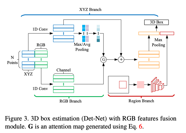
    predict the center δ of RoI using a lightweight network and use it to update the point cloud as follow:

    $$S^{\prime \prime}=\left\{p \mid p-\delta, p \in S^{\prime}\right\}$$

    Estimate here is a ’residual’ center, which means the real center is C + δ.

    RGB Information Aggregation: aggregate complementary RGB information to point cloud.

    $$S=\{p \mid p \leftarrow \mathbf{F}(v), D(v), v \in \mathbf{B}\}$$

    D is a function which output the corresponding RGB values of input point. 6D vectors: [x, y, z, r, g, b].

    utilize the attention mechanism for guiding the message passing between the spatial features and RGB features. the attention can act as a gate function.

    An attention map G is first produced from the feature maps F generated from XYZ branch as follow:

    $$\mathbf{G} \leftarrow \sigma\left(f\left(\left[\mathbf{F}_{\max }^{x y z}, \mathbf{F}_{a v g}^{x y z}\right]\right)\right)$$

    f is the nonlinear function learned from a convolution layer and σ is a sigmoid function for normalizing the attention map.

    $$\mathbf{F}^{x y z} \leftarrow \mathbf{F}^{x y z}+\mathbf{G} \odot \mathbf{F}^{r g b}$$

simultaneously optimize the two networks for 3D detection jointly with a multi-task loss function:

$$L=L_{loc}+L_{det}+\lambda L_{corner}$$

---

Backwards:

Because it’s a 2D-driven framework, the proposed method will fail if the 2D box is a false positive sample or missing.

MonoDIS: Disentangling Monocular 3D Object Detection——2019

Disentangling transformation for 2D and 3D detection losses and a novel, self-supervised confidence score for 3D bounding boxes. Our proposed loss disentanglement has the twofold advantage of simplifying the training dynamics in the presence of losses with complex interactions of parameters, and sidestepping the issue of balancing independent regression terms. Our solution overcomes these issues by isolating the contribution made by groups of parameters to a given loss, without changing its nature.

本文的核心是提出了解耦的 regression loss，用来替代之前同时回归 center、size、rotation 带来的由于各个 opponent 的 loss 大小不同导致的训练问题；基本思想是将回归的部分分成 k 个 group，每个 group 只有自身的参数需要学习，其他的部分使用 gt 代替，从而实现每个分支只回归某一个 component，使得训练更加稳定。同时提出了改进的 sIoU loss，将没有 overlap 的 bboxes 的 loss 也考虑进来。同时，本文使用 memory efficient in-place synced bn 替换了原来的 BatchNorm，从而更 efficient 的训练；

这么一看，这篇文章解决了我的很多问题，第一个问题回归三个信息的大小不同问题，在我的实验时也发现了此问题，但是我的解决方案就是简单地用函数包装一些信息，使得他们的范围相差不大；但是这样做实际上是将大范围的预测变得粗略化了；第二个问题，改进的sIoU loss，这一个问题是被学长提问的时候发现的，我对这一段的处理是采用了2D检测的方法，有了Prec来表示，在训练时用heatmap的loss来计算，但是这样做，在评估的时候相当于多个独立的评估，不在一个整体之中，而且对于loss之间的一个weight问题相当于不用考虑？；第三个问题阅读之前还是不清楚是什么问题。这么一看2019年的文章，这些问题我可以发现，但是我没有去思考一个更好的方法，而是去找个短暂的解决方案。

---

Backbone:

2D Detection Head:

其中，在2D bounding box的置信度为$p\in[0,1]$

$$p_{2 \mathrm{D}}=\left(1+e^{-\zeta_{2 \mathrm{D}}}\right)^{-1}$$

分析可得，$\zeta_{2 \mathrm{D}}$趋向于正无穷时，置信度趋向于1；但$\zeta_{2 \mathrm{D}}$趋向于负无穷时，置信度趋向于0。

根据图像坐标系分成的cell g的中心点为$(u_g, v_g)$， 那么bounding box的中心点为

$$\left(u_{b}, v_{b}\right)=\left(u_{g}+\delta_{u} w_{a}, v_{g}+\delta_{v} h_{a}\right)$$

bounding box的大小为

$$\left(w_{b}, h_{b}\right)=\left(w_{a} e^{\delta w}, h_{a} e^{\delta_{h}}\right)$$

Use focal loss to train the bounding box confidence score.

$$L_{2 \mathrm{D}}^{\mathrm{conf}}\left(p_{2 \mathrm{D}}, y\right)=-\alpha y\left(1-p_{2 \mathrm{D}}\right)^{\gamma} \log p_{2 \mathrm{D}}-\bar{\alpha} \bar{y} p_{2 \mathrm{D}}^{\gamma} \log \left(1-p_{2 \mathrm{D}}\right)\\ \bar \alpha=1-\alpha,\quad \bar y=1-y$$

其中，y是target confidence $y\in \{0, 1\}$. $\alpha\in[0,1], \gamma>0$超参数。

Detection loss:

$$L_{2 \mathrm{D}}^{\mathrm{bb}}(\boldsymbol{b}, \hat{\boldsymbol{b}})=1-\operatorname{sIoU}(\boldsymbol{b}, \hat{\boldsymbol{b}})$$ $$\operatorname{sIoU}(\boldsymbol{b}, \hat{\boldsymbol{b}})=\frac{|\boldsymbol{b} \sqcap \hat{\boldsymbol{b}}|_{\pm}}{|\boldsymbol{b}|+|\hat{\boldsymbol{b}}|-|\boldsymbol{b} \sqcap \hat{\boldsymbol{b}}|_{\pm}}$$

where

$$\boldsymbol{b} \sqcap \hat{\boldsymbol{b}}=\left(\begin{array}{c} \max \left(u_{1}, \hat{u}_{1}\right) \\ \max \left(v_{1}, \hat{v}_{1}\right) \\ \min \left(u_{2}, \hat{u}_{2}\right) \\ \min \left(v_{2}, \hat{v}_{2}\right) \end{array}\right)$$

b是bounding box. sIoU represents an extension of the common IoU function, which prevents gradients from vanishing in case of non-overlapping bounding boxes. call it signed IoU.

其中正负号定义：

$$|\boldsymbol{b}|_{\pm}=\left\{\begin{array}{ll} +|\boldsymbol{b}| & \text { if } u_{2}>u_{1} \text { and } v_{2}>v_{1} \\ -|\boldsymbol{b}| & \text { otherwise } \end{array}\right.$$

3D Detection Head:

$$\theta=\left(\delta z, \Delta_{u}, \Delta_{v}, \delta_{W}, \delta_{H}, \delta_{D}, q_{r}, q_{i}, q_{j}, q_{k}\right)$$

其中，对于给出的2D proposal预测的3D bounding box的置信度为【公司不能用，应该是因为3D信息的标注并不是对于全部object；并且其真实置信度是根据能学习到的bbox来确定的】

$$p_{3 \mathrm{D} \mid 2 \mathrm{D}}=\left(1+e^{-\zeta_{3 \mathrm{D}}}\right)^{-1}$$

中心点的深度

$$z=\mu_z+\sigma_z\delta_z$$

中心点在图像上的投影位置

$$c=(u_b+\Delta_u,v_b+\Delta_v)$$

3D大小同样也是有先验值的基础上的

$$\boldsymbol{s}=\left(W_{0} e^{\delta_{W}}, H_{0} e^{\delta_{H}}, D_{0} e^{\delta_{D}}\right)$$

pose

$$\boldsymbol{q}=q_{r}+q_{i} \mathrm{i}+q_{j} \mathrm{j}+q_{k} \mathrm{k}$$

Detection loss:

$$L_{3 \mathrm{D}}^{\mathrm{bb}}(\boldsymbol{B}, \hat{\boldsymbol{B}})=\frac 1 8\|B-\hat B\|_H$$

其中，$\|\cdot\|_H$ denotes the Huber loss.

对于3D置信度预测的损失，则是通过自主学习，计算它的loss仍然通过the standard binary cross entropy loss；它的真实值通过一个转换得到

$$\hat{p}_{3 \mathrm{D} \mid 2 \mathrm{D}}=e^{-\frac{1}{T} L_{3 \mathrm{D}}^{\mathrm{bb}}(B, \hat{B})}\\ L_{3 \mathrm{D}}^{\mathrm{conf}}\left(p_{3 \mathrm{D} \mid 2 \mathrm{D}}, \hat{p}_{3 \mathrm{D} \mid 2 \mathrm{D}}\right)=-\hat{p} \log p-(1-\hat{p}) \log (1-p)$$

根据贝叶斯，可以得到3D置信度：

$$p_{3D}=p_{3D|2D}p_{2D}$$

这样在预测阶段的时候，通过阈值$\tau_{conf}$过滤掉框，后面就不用NMS或者3D先验知识后处理了。

---

Car size of $W_0 = 1.53m, H_0 = 1.63m, D_0 = 3.88m$ and depth statistics of $\mu_z = 28.01m$ and $\sigma_ z = 16.32m$. We filtered the final 3D detections with a score threshold of $\tau_{conf} = 0.05$.

GS3D: An Efficient 3D Object Detection Framework for Autonomous Driving——2019

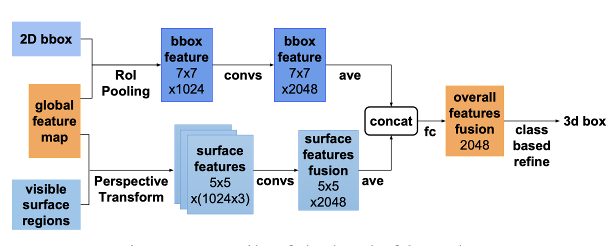
Leveraging the off-the-shelf 2D object detector, we propose an artful approach to efficiently obtain a coarse cuboid for each predicted 2D box. The coarse cuboid has enough accuracy to guide us to determine the 3D box of the object by refinement. we explore the 3D structure information of the object by employing the visual features of visible surfaces.

---

• 首先用成熟的2D检测器，得到2Dbbox、类别和方向；

  

• 然后确定它的basic cuboid；

• 最后从可见的面上提取特征，进行refinement

  从可见面上提取而不是2D框上提取是因为，相同2D框不同朝向的cubic应该有不同的置信度。

  可见面的表面特征用了数据增强；因为同一个bbox的朝向是很重要的

Discrete classification based methods with quality aware loss(the more accurate target box gets the higher score) perform much better than direct regression approaches for the task of 3D box refinement.

$$q=\left\{\begin{array}{ll} 1 & \text { if } o v>0.75 \\ 0 & \text { if } o v<0.25 \\ 2 o v-0.5 & \text { otherwise } \end{array}\right.$$

ov is the 3D overlap between the target box and ground-truth.

• dimension可以根据2Dbbox生成的类别信息，得到一个先验的值。
• 根据2D bbox顶部和底部的中心点，可以得到3D坐标下归一化的坐标值，从而高。底部中心点上增加了一个微小的抖动，由统计得到。
• 朝向角根据观察角加上位置偏向角的和得到。
• 根据角度，对应的可见面就可以得到。大于0说明正面可见，小于零的说明背面可见，在$(-\frac \pi 2,\frac \pi 2)$左面可见，剩下的就是右面可见。
• 回归残差问题转变为分类问题，bin-loss

use BCE as the loss function

$$L_{q u a l i t y}=-[q \log (p)+(1-q) \log (1-p)]$$

something

要去了解的方法：

• Part-sensitive warping预测框不匹配的方法
• Frustum-PointNet（F-PointNet视锥）
• AVOD

转载请注明出处，谢谢。

愿 我是你的小太阳