Machine Learning-regression model

This is my blog.

回归模型

应该算是最基础的吧

梯度下降法,之后也用的比较多

幸好之前也选修了数值分析

对这些东西还算有了解啦!

这里只要有两种,一种是线性回归,另一种是逻辑回归

遇到了一个函数,sigmoid,这个函数还是很神奇哒!

Octave集成的也很棒,Matlab也很棒啦!

打算学完之后,用python巩固一下

好像看到班里的大大们,都是用python研究的么!

Lesson 2 liner regression
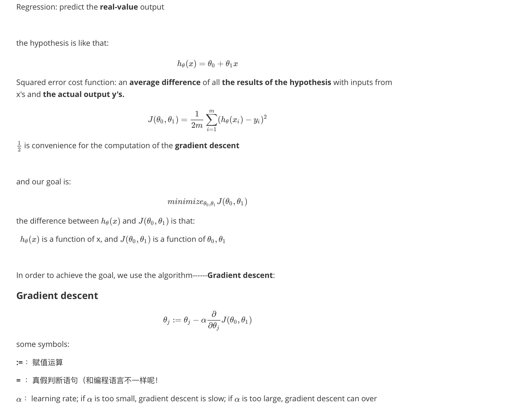
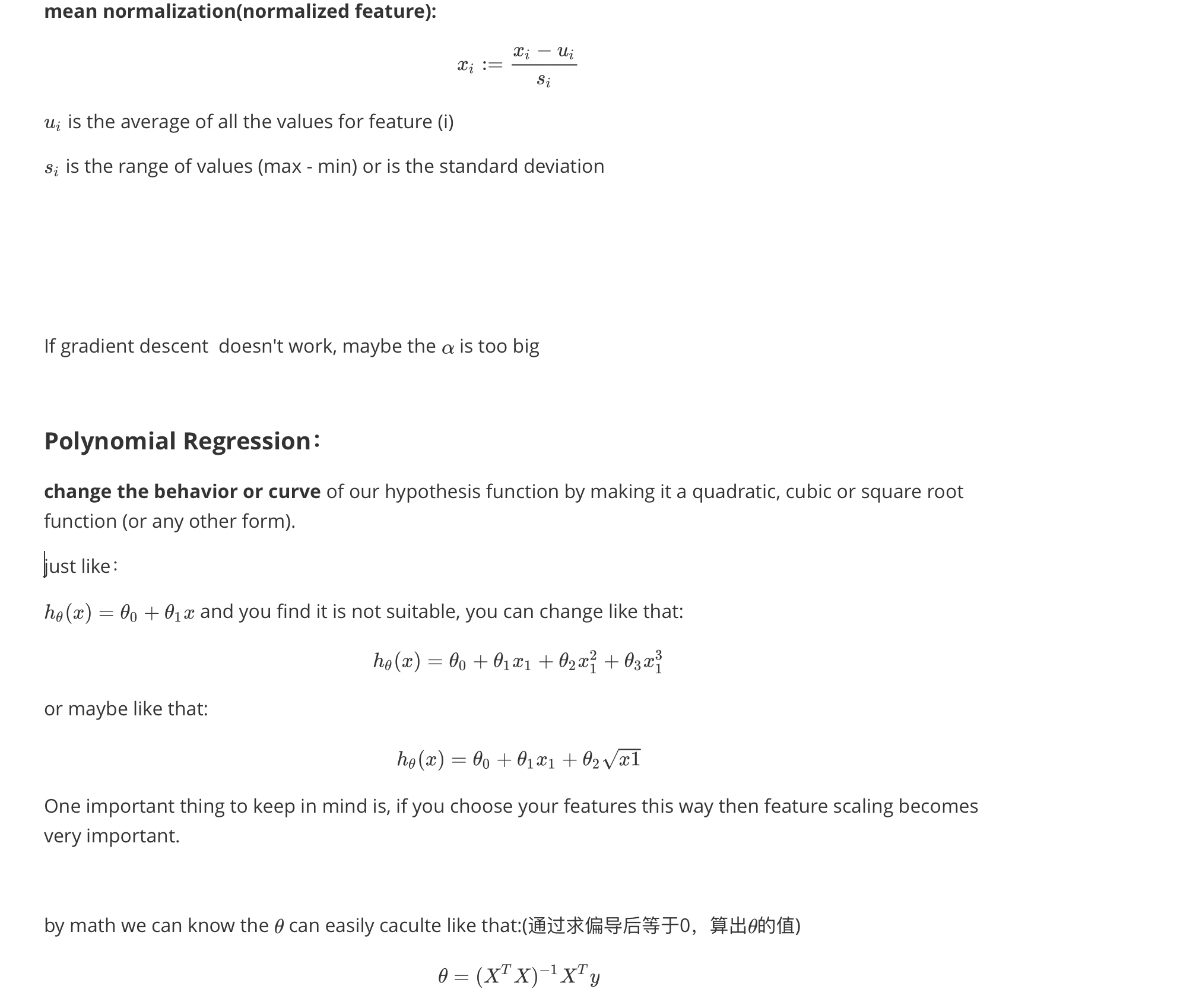
shootthe minimum. It may fail to converge, or even diverge.

Attention: In the updating, we should simultaneously update both the parameters $\theta_0$ and $\theta_1 $

The closer is, the slower is.

problem: you may find local minimum, not the global minimum. But in the liner regression, the figure is like a bowl, so the problem will not happened.

“Batch” gradient descent: which says each steps of gradient descent uses all of training examples

Matrix: Dimension of matrix: rows columns (nm)

Vector: an n*1 matrix

Lesson 3 multivariate Liner regression
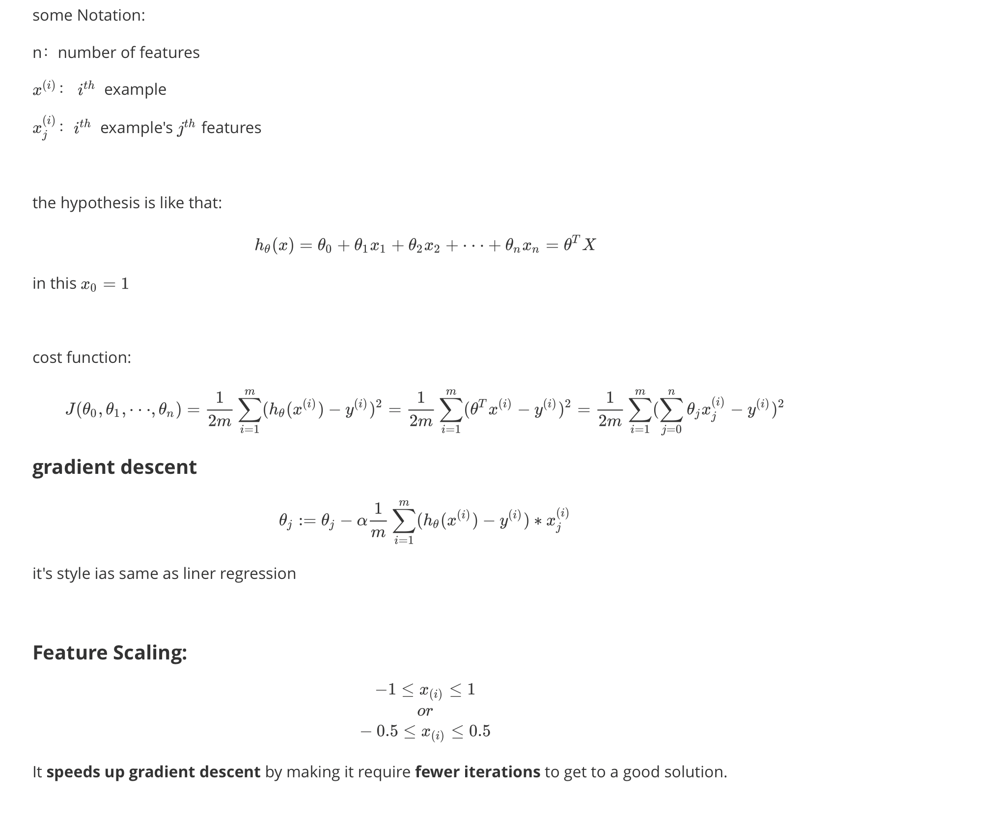
In octave:

1
pinv(x' * x) * x' * y

The ‘pinv’ function will give you a value of θ even if $X^TX)\ is not invertible.[if you use the inv(), then you will get error! ]

And the reasons for the “not invertible” are:

  • Redundant features, where two features are very closely related (i.e. they are linearly dependent)
  • Too many features (e.g. m ≤ n). In this case, delete some features or use “regularization” (正则化)

But the two ways have both advantages and disadvantages :

and in other more complicated problems we will find the gradient descent is more useful.

In practice, when n exceeds 10,000 it might be a good time to go from a normal solution to an iterative process.

Lesson 4 Octave

In octave, the index is not from “0”, but from “1”.

Basics :

1
2
3
4
5
6
7
8
9
10
11
12
13
14
15
16
17
18
19
20
21
22
23
24
25
26
27
28
29
PS1(">> ")
a=pi
disp(sprintf("%.6f",a))
disp("hello\n")
who % all the variables in the workplace
whos %like who, but give you details
% something like cmd
pwd
cd 'C:\'
ls
clear
addpath('C:\')
% something like matlab
format long
format short
rand(3) % 3*3
rand(1,2) % 0到1之前的随机值
randn(1,2) % 平均值为0,平均方差为1的高斯随机值
A(2,:) % : means every elements in 2th row
A([1 3],:) % all the elements in the first and third row
A(:) % but in this answer, the ans will be in a vector, not like the matrix
A = [1;2]
size(A) % 2 1
length(A) % 2;the longest size

Input data:

1
2
3
4
5
6
7
load('file_name.dat')
load 'file_name.dat'
file_name % see the data
save name.mat V %put the V into the 'name.data'
save name.txt V -ascii % save as txt, and you can see the result only by open the txt

Computing:

1
2
3
4
5
6
7
8
9
10
11
12
13
14
15
16
17
18
19
20
21
22
23
24
25
26
27
28
29
A*B % can not write like that "AB"
A+2 % every element add 2
x/2 % every element divide 2
x.^2 % every element multiply themself, not same as x^2
A .* B % 矩阵哈达马积,对应元素相乘
A .^ 2 % every element to multiple 2
exp(V)
log(V)
abs(V)
val = max(A)
[val,index] = max(A)
find(V<3) % the index of V's elements that smaller than 3
[r,c] = find(A<3)
magic(x) % x*x matrix, and the sum of every rows, column, diagonals is same
sum(A)
floor(A)
ceil(A)
prod(A) % all the elements multiply together
max(A,[],x) %find the max in every x columns
sum(A,1) % the sum of every column
sum(A,2) % the sum of every row
filpud(A) %上下翻转
pinv(A) % inv(A)

Plotting:

1
2
3
4
5
6
7
8
9
10
11
12
13
14
15
16
17
18
19
20
21
22
23
24
25
26
27
28
29
30
plot(x,y);
% do something with firgure
plot(x,y1,'r')
plot(x,y2,'b')
hold on;
xlabel('x')
ylabel('y')
title('title')
legend('y1','y2')
print -dpng 'myplot.png'
% also can change the path like that
cd 'C:/' print -dpng 'myplot.png'
close
figure(1);plot(x,y1,'r')
figure(2);plot(x,y2,'b')
subplot(1,2,1) %divides plot 1*2 grid, access element 1
plot(x,y1,'r')
subplot(1,2,2)
plot(x,y2,'b')
axis([0.5 1 -1 1]) % x[0.5 1] y[-1 1] for subplot(1,2,2)
clf; % clear figure
% other figure
imagesc(A)
imagesc(A),colorbar,colormap gray

Control:

1
2
3
4
5
6
7
8
9
10
11
12
for i=1:10,
% ....
end;
if
elseif
else
end;
function y=functionname(X)
y=x^2

if you can use the vector, try to use it to cacluate which will decrease the length of code.

Lesson 5 Classfication
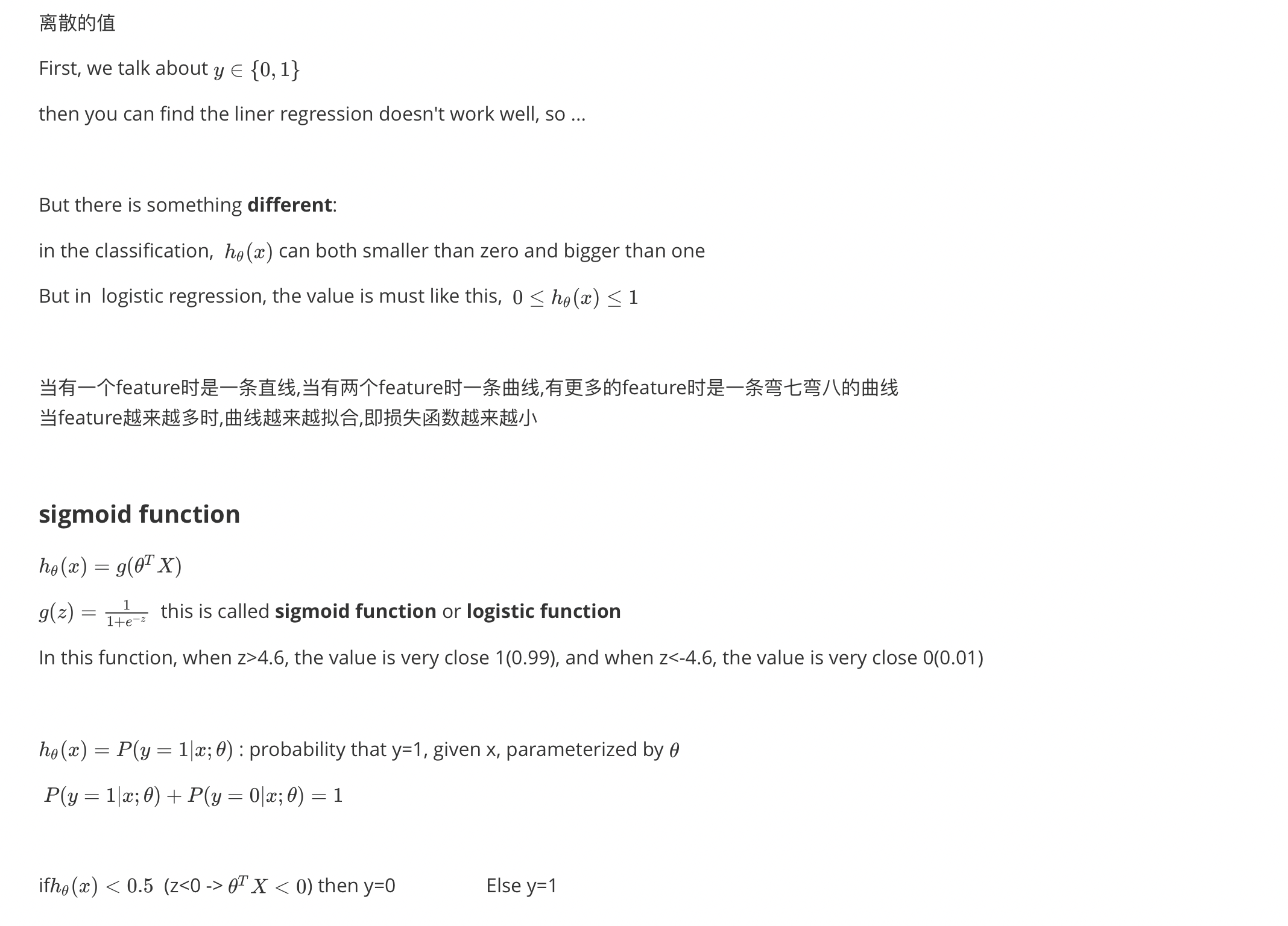
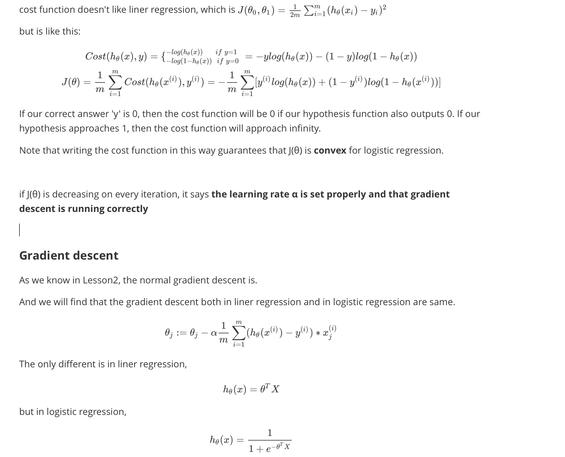
Lesson 6 Logistic Regression Model
1
2
3
4
5
6
7
8
function [jVal, gradient] = costFunction(theta)
jVal = [...code to compute J(theta)...];
gradient = [...code to compute derivative of J(theta)...];
end
options = optimset('GradObj', 'on', 'MaxIter', 100);
initialTheta = zeros(2,1);
[optTheta, functionVal, exitFlag] = fminunc(@costFunction, initialTheta, options);

There are other three ways to solve it, and these ways are more faster and you don’t need find the optimal α by manually. But it is more complex. (It isn’t because it will lost in local minimum)

Conjuate gradient

BFGS

L-BFGS

Multiclass Classification

后记

上交完实验后,还是很开心哒!

不过我居然在绿色计算机大赛的时候

犯了小迷糊

可能那一天都在迷糊吧

转载请注明出处,谢谢。

愿 我是你的小太阳

买糖果去喽