Neural Networks and Deep Learning

This is my blog.

新的一门课开始啦～

感觉还不错啦～

新的一门课，找首新歌吧～

Suggestion

• 多读文献
• 编程
• 培养自己的直觉，并且相信自己的直觉

What is Neural Nerworks

激活函数

具体可见之间文章手写数字识别

每层的激活函数可以不同

• 线性整流函数(Rectified linear unit) RELU

  但是在负数的时候，导数为0；因此出现了leaky Relu，eg.max(0.01z,z), the 0.01 can change，但后者不常使用

  max(0,y)

  

• 达到数据中心化的效果

  一般来说，效果比sigmoid更好

激活函数一般不用线性的，或者不用不用（就是$g(z)=z$）

这样会使隐藏层没有存在的意义，也就是说神经网络和没有学习能力一样，只存在着线性的惯性，多步可以合成一个大点的线性关系；

线性激活函数一般用在输出层，用来预测房价类型的问题

Structured Data

给出结构化数据，每一个特征都有清晰的定义

每一个特征都有明确的数值

Unstructured Data

非结构的，例如音频，图片，文字

The iterative process of developing DL systems： Idea->Code->Experiment->Idea->….

NN

之后的博文会更新，更新完后，会在此加上链接

• Standard NN
• CNN
• RNN

Logistics Regression as a neural network

It is a Binary classification （二分类问题）

这里只有两层（输入层不算）

在Regression Model-Lesson6提到过一些概念，现大致重述如下：

optimization

vectorization

在python的numpy包中有许多内置函数，可以进行并行运算，比for循环更快

You can get time running time of one programm is to use time.time() method in package time. 单位10^{-6}s

一些内置函数

cal = A.sum(axis=0) # 列求和，行压缩
np.log(A, B)
np.exp(A, B) # the "math" library in deep learning because the inputs of the functions are real numbers. In deep learning we mostly use matrices and vectors. This is why numpy is more useful.

# 对于以下三种乘法，我将重点分析一下区别
A * B # 会进行广播原则，对应元素相乘

np.dot(A, B) # For 2-D arrays it is equivalent to matrix multiplication, and for 1-D arrays to inner product of vectors (without complex conjugation)【对应元素相乘再相加，见下面例子中的np.dot(c, a).而若A，B是matrix的时候，则需要大小满足矩阵相乘的条件

np.multiply(A, B) # 对应元素相乘，当矩阵的维度不相同时，会根据一定的广播规则将维数扩充到一致的形式. 如果不能广播相同的size，multiply就会失败

x_norm = np.linalg.norm(x, ord =2, axis=1, keepdims=True) # 求范式
# ord几范式（默认二范式） 一范式：|x1|+...+|xn|	二范式：sqrt(x1^2+...+xn^2) 无穷范式: max(|xi|)
# axis=1表示按行向量处理，求多个行向量的范数；axis=0表示按列向量处理，求多个列向量的范数；axis=None表示矩阵范数
# keepdims True表示保持矩阵的二维特性，False相反

给一下测试的结果

>>> a = np.array([1, 2, 3])  # (3,)
array([1, 2, 3]) 	
>>> b = np.array([[1, 2,3]]) # (1,3)
array([[1, 2, 3]])	
>>> c = np.array([[4, 5, 6],[7, 8, 9]]) # (2,3)
array([[4, 5, 6], 
       [7, 8, 9]])		

# A * B 
>>> print(a*b) # 对应元素相乘
[[1 4 9]]
>>> print(a*c) # 先进行广播原则，再对应元素相乘
[[ 4 10 18]
 [ 7 16 27]]
>>> print(c*a) # 先进行广播原则，再对应元素相乘
[[ 4 10 18]
 [ 7 16 27]]
>>> print(b*c) # 先进行广播原则，再对应元素相乘
[[ 4 10 18]
 [ 7 16 27]]
>>> print(c*b) # 先进行广播原则，再对应元素相乘
[[ 4 10 18]
 [ 7 16 27]]
>>> print(b*a) # 先进行广播原则，再对应元素相乘
[[1 4 9]]

# np.dot(A, B)
>>> print(np.dot(a,b)) # 不满足矩阵相乘概念 a(3,) b(1,3)注意a只是秩为1，它的shape很神奇哦
Traceback (most recent call last):
  File "<pyshell#32>", line 1, in <module>
    print(np.dot(a,b))
ValueError: shapes (3,) and (1,3) not aligned: 3 (dim 0) != 1 (dim 0)
>>> print(np.dot(b,a)) # b(1,3) a(3, ) 
[14]
>>> print(np.dot(a,c)) # 不满足矩阵相乘概念 a(3,) c(2,3)
Traceback (most recent call last):
  File "<pyshell#34>", line 1, in <module>
    print(np.dot(a,c))
ValueError: shapes (3,) and (2,3) not aligned: 3 (dim 0) != 2 (dim 0)
>>> print(np.dot(c, a)) # c(2,3) a(3,)得到的不是两行哦！32=1*4+2*3*6	50=1*7+2*8+3*9
[32 50]
>>> print(np.dot(b,c)) # 不满足矩阵相乘概念 b(1,3) c(2,3)
Traceback (most recent call last):
  File "<pyshell#36>", line 1, in <module>
    print(np.dot(b,c))
ValueError: shapes (1,3) and (2,3) not aligned: 3 (dim 1) != 2 (dim 0)
>>> print(np.dot(c,b)) # 不满足矩阵相乘概念 c(2,3) b(1,3)
Traceback (most recent call last):
  File "<pyshell#37>", line 1, in <module>
    print(np.dot(c,b))
ValueError: shapes (2,3) and (1,3) not aligned: 3 (dim 1) != 1 (dim 0)
>>> np.dot(c,b.T) # c(2,3) b.T(3,1) 矩阵运算
array([[32],
       [50]])

# np.multiply(A, B)
>>> print(np.multiply(a,b)) # a(3, ) b(1,3)对应元素相乘
[[1 4 9]]
>>> print(np.multiply(b,a)) # b(1,3) a(3, )对应元素相乘
[[1 4 9]]
>>> print(np.multiply(a,c)) # a(3, ) c(2,3)对应元素相乘
[[ 4 10 18]
 [ 7 16 27]]
>>> print(np.multiply(c,a)) # c(2,3) a(3, )对应元素相乘
[[ 4 10 18]
 [ 7 16 27]]
>>> print(np.multiply(b,c)) # 先进行广播原则，再对应元素相乘
[[ 4 10 18]
 [ 7 16 27]]
>>> print(np.multiply(c,b)) # 先进行广播原则，再对应元素相乘
[[ 4 10 18]
 [ 7 16 27]]

在python中，若是一个向量加上一个常数，那么就等同于一个向量加上一个同样大小的向量，并且这个向量的值都是这个常数，这叫作broadcasting

因此现在我们可以将方法二的进行向量化

import numpy as np
for i in range(iterations):
    # 前向传播
	Z = np.dot(W.T, X) # X (n_x * m) W (n_x * 1)
	A = sigma(Z) # A (1 * m)
    #反向传播
	dZ = A - Y # Y (1 * m)
	dW = 1 / m * X * dZ.T # dW (n_x * 1)
	db = 1 / m * np.sum(dZ) # db (1 * 1)
    # 梯度下降
    W = W - alpha * dW
    b = b - alpha * db

接下来，我们来了解一下python中的broadcasting

当array的时候，(m,n) 要[+,-,*,/] (1,n)或者(m,1)的向量的时候，后者会扩展为(m,n)的向量，再进行运算

注意当用array创建的时候，用np.random.randn(5,1)而不是np.random.randn(5)，前者创建的是矩阵，后者创建的是秩为1的数组；后者是形如[[1, 2, 3]]前者是[1, 2, 3]

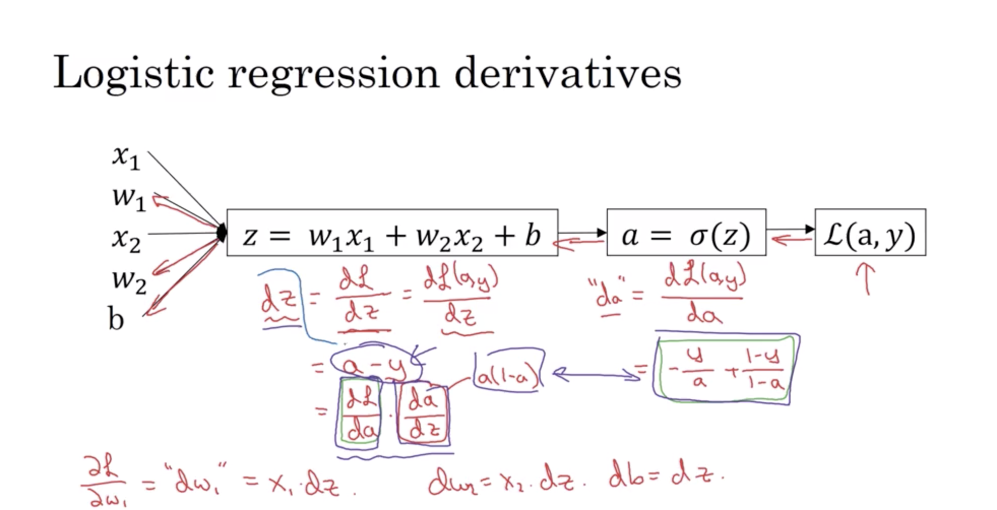
Computation graph

正向流程图，forward to compute the cost function

One step of backward propagation on a computation graph yields derivative of final output variable.后向计算导数，优化代价函数

链式法则：感觉有点像蝴蝶效应（我瞎说的，就是一种影响的传播

python

建议完成课程后的作业，感觉代码很棒呢！

# GRADED FUNCTION: sigmoid
def sigmoid(z):
    """
    Compute the sigmoid of z

    Arguments:
    z -- A scalar or numpy array of any size.

    Return:
    s -- sigmoid(z)
    """

    s = 1 / (1 + np.exp(-z))

    return s



# GRADED FUNCTION: initialize_with_zeros

def initialize_with_zeros(dim):
    """
    This function creates a vector of zeros of shape (dim, 1) for w and initializes b to 0.

    Argument:
    dim -- size of the w vector we want (or number of parameters in this case)

    Returns:
    w -- initialized vector of shape (dim, 1)
    b -- initialized scalar (corresponds to the bias)
    """

    w = np.zeros((dim, 1))
    b = 0

    assert (w.shape == (dim, 1))
    assert (isinstance(b, float) or isinstance(b, int))

    return w, b


# GRADED FUNCTION: propagate

def propagate(w, b, X, Y):
    """
    Implement the cost function and its gradient for the propagation explained above

    Arguments:
    w -- weights, a numpy array of size (num_px * num_px * 3, 1)
    b -- bias, a scalar
    X -- data of size (num_px * num_px * 3, number of examples)
    Y -- true "label" vector (containing 0 if non-cat, 1 if cat) of size (1, number of examples)

    Return:
    cost -- negative log-likelihood cost for logistic regression
    dw -- gradient of the loss with respect to w, thus same shape as w
    db -- gradient of the loss with respect to b, thus same shape as b

    Tips:
    - Write your code step by step for the propagation. np.log(), np.dot()
    """

    m = X.shape[1]

    # FORWARD PROPAGATION (FROM X TO COST)
    A = sigmoid(np.dot(w.T, X) + b)  # compute activation
    cost = - 1 / m * np.sum(Y * np.log(A) + (1 - Y) * np.log((1 - A)))  # compute cost

    # BACKWARD PROPAGATION (TO FIND GRAD)
    dw = 1 / m * np.dot(X, (A - Y).T)
    db = 1 / m * np.sum((A - Y))

    assert (dw.shape == w.shape)
    assert (db.dtype == float)
    cost = np.squeeze(cost)
    assert (cost.shape == ())

    grads = {"dw": dw,
             "db": db}

    return grads, cost



# GRADED FUNCTION: optimize

def optimize(w, b, X, Y, num_iterations, learning_rate, print_cost=False):
    """
    This function optimizes w and b by running a gradient descent algorithm

    Arguments:
    w -- weights, a numpy array of size (num_px * num_px * 3, 1)
    b -- bias, a scalar
    X -- data of shape (num_px * num_px * 3, number of examples)
    Y -- true "label" vector (containing 0 if non-cat, 1 if cat), of shape (1, number of examples)
    num_iterations -- number of iterations of the optimization loop
    learning_rate -- learning rate of the gradient descent update rule
    print_cost -- True to print the loss every 100 steps

    Returns:
    params -- dictionary containing the weights w and bias b
    grads -- dictionary containing the gradients of the weights and bias with respect to the cost function
    costs -- list of all the costs computed during the optimization, this will be used to plot the learning curve.

    Tips:
    You basically need to write down two steps and iterate through them:
        1) Calculate the cost and the gradient for the current parameters. Use propagate().
        2) Update the parameters using gradient descent rule for w and b.
    """

    costs = []

    for i in range(num_iterations):

        # Cost and gradient calculation (≈ 1-4 lines of code)
        grads, cost = propagate(w, b, X, Y)

        # Retrieve derivatives from grads
        dw = grads["dw"]
        db = grads["db"]

        # update rule (≈ 2 lines of code)
        w = w - learning_rate * dw
        b = b - learning_rate * db

        # Record the costs
        if i % 100 == 0:
            costs.append(cost)

        # Print the cost every 100 training iterations
        if print_cost and i % 100 == 0:
            print("Cost after iteration %i: %f" % (i, cost))

    params = {"w": w,
              "b": b}

    grads = {"dw": dw,
             "db": db}

    return params, grads, costs


# GRADED FUNCTION: predict

def predict(w, b, X):
    '''
    Predict whether the label is 0 or 1 using learned logistic regression parameters (w, b)

    Arguments:
    w -- weights, a numpy array of size (num_px * num_px * 3, 1)
    b -- bias, a scalar
    X -- data of size (num_px * num_px * 3, number of examples)

    Returns:
    Y_prediction -- a numpy array (vector) containing all predictions (0/1) for the examples in X
    '''

    m = X.shape[1]
    Y_prediction = np.zeros((1, m))
    w = w.reshape(X.shape[0], 1)

    # Compute vector "A" predicting the probabilities of a cat being present in the picture
    ### START CODE HERE ### (≈ 1 line of code)
    A = sigmoid(np.dot(w.T, X) + b)
    ### END CODE HERE ###

    for i in range(A.shape[1]):

        # Convert probabilities A[0,i] to actual predictions p[0,i]
        ### START CODE HERE ### (≈ 4 lines of code)
        if A[0, i] > 0.5:
            Y_prediction[0, i] = 1
        ### END CODE HERE ###

    assert (Y_prediction.shape == (1, m))

    return Y_prediction


# GRADED FUNCTION: model

def model(X_train, Y_train, X_test, Y_test, num_iterations=2000, learning_rate=0.5, print_cost=False):
    """
    Builds the logistic regression model by calling the function you've implemented previously

    Arguments:
    X_train -- training set represented by a numpy array of shape (num_px * num_px * 3, m_train)
    Y_train -- training labels represented by a numpy array (vector) of shape (1, m_train)
    X_test -- test set represented by a numpy array of shape (num_px * num_px * 3, m_test)
    Y_test -- test labels represented by a numpy array (vector) of shape (1, m_test)
    num_iterations -- hyperparameter representing the number of iterations to optimize the parameters
    learning_rate -- hyperparameter representing the learning rate used in the update rule of optimize()
    print_cost -- Set to true to print the cost every 100 iterations

    Returns:
    d -- dictionary containing information about the model.
    """
    
    # initialize parameters with zeros (≈ 1 line of code)
    w, b = initialize_with_zeros(X_train.shape[0])

    # Gradient descent (≈ 1 line of code)
    parameters, grads, costs = optimize(w, b, X_train, Y_train, num_iterations, learning_rate, print_cost)

    # Retrieve parameters w and b from dictionary "parameters"
    w = parameters["w"]
    b = parameters["b"]

    # Predict test/train set examples (≈ 2 lines of code)
    Y_prediction_test = predict(w, b, X_test)
    Y_prediction_train = predict(w, b, X_train)

    ### END CODE HERE ###

    # Print train/test Errors
    print("train accuracy: {} %".format(100 - np.mean(np.abs(Y_prediction_train - Y_train)) * 100))
    print("test accuracy: {} %".format(100 - np.mean(np.abs(Y_prediction_test - Y_test)) * 100))

    d = {"costs": costs,
         "Y_prediction_test": Y_prediction_test,
         "Y_prediction_train": Y_prediction_train,
         "w": w,
         "b": b,
         "learning_rate": learning_rate,
         "num_iterations": num_iterations}

    return d



# Loading the data (cat/non-cat)
train_set_x_orig, train_set_y, test_set_x_orig, test_set_y, classes = load_dataset()

# get the information of sets
m_train = train_set_x_orig.shape[0]
m_test = test_set_x_orig.shape[0]
num_px = train_set_x_orig.shape[1]
# Reshape the training and test examples
# A trick when you want to flatten a matrix X of shape (a,b,c,d)
# to a matrix X_flatten of shape (b ∗∗ c ∗∗ d, a) is to use:
# X_flatten = X.reshape(X.shape[0], -1).T      # X.T is the transpose of X

train_set_x_flatten = train_set_x_orig.reshape(train_set_x_orig.shape[0], -1).T
test_set_x_flatten = test_set_x_orig.reshape(test_set_x_orig.shape[0], -1).T

# standardize dataset
train_set_x = train_set_x_flatten/255.
test_set_x = test_set_x_flatten/255.

# test learning rates
learning_rates = [0.01, 0.001, 0.0001]
models = {}
for i in learning_rates:
    print ("learning rate is: " + str(i))
    models[str(i)] = model(train_set_x, train_set_y, test_set_x, test_set_y, num_iterations = 1500, learning_rate = i, print_cost = False)
    print ('\n' + "-------------------------------------------------------" + '\n')

for i in learning_rates:
    plt.plot(np.squeeze(models[str(i)]["costs"]), label= str(models[str(i)]["learning_rate"]))

plt.ylabel('cost')
plt.xlabel('iterations (hundreds)')

legend = plt.legend(loc='upper center', shadow=True)
frame = legend.get_frame()
frame.set_facecolor('0.90')
plt.show()


# predict new pictures
my_image = "avatar.jpg"   # change this to the name of your image file
fname = "images/" + my_image
image = np.array(ndimage.imread(fname, flatten=False))
my_image = scipy.misc.imresize(image, size=(num_px,num_px)).reshape((1, num_px*num_px*3)).T
d = model(train_set_x, train_set_y, test_set_x, test_set_y, num_iterations = 2000, learning_rate = 0.005, print_cost = True)
my_predicted_image = predict(d["w"], d["b"], my_image)

plt.imshow(image)
print("y = " + str(np.squeeze(my_predicted_image)) + ", your algorithm predicts a \"" + classes[int(np.squeeze(my_predicted_image)),].decode("utf-8") +  "\" picture.")

Standard NN(标准神经网络)

The general methodology to build a Neural Network is to:

1. Define the neural network structure ( # of input units, # of hidden units, etc).
2. Initialize the model’s parameters
3. Loop:
   • Implement forward propagation
   • Compute loss
   • Implement backward propagation to get the gradients
   • Update parameters (gradient descent)

逻辑回归模型中，可以初始化为0，因为：

Logistic Regression doesn’t have a hidden layer. If you initialize the weights to zeros, the first example x fed in the logistic regression will output zero but the derivatives of the Logistic Regression depend on the input x (because there’s no hidden layer) which is not zero. So at the second iteration, the weights values follow x’s distribution and are different from each other if x is not a constant vector.

但是在神经网络中不可以，因为这样隐藏单元会一直是同样的功能，即隐藏神经元是对称的

由w影响的的，所以b可以初始化为0

而w则需使用np.random.randn()，同时，将这个生成的数，乘以一个较小的值，如0.01，这样通过计算得到的z绝对值较小，在激活函数中的斜率比较大，学习速率就可以大些。

同时每一层乘的数最好不相同。

在编程的时候，对于每一个变量最好写上shape

第一层网络一般被认为是特征检测器

the “cache” records values from the forward propagation units and sends it to the backward propagation units because it is needed to compute the chain rule derivatives.

Hyperparameters 超参数

都会影响W和b

• learning rate
• Iteration
• Hidden layers
• Hidden units
• choice of activation function

在其他神经网络中我们还会遇到的超参数：

• Momentum term
• Mini batch size
• Regularizations Parameters
• ……

注：The deeper layers of a neural network are typically computing more complex features of the input than the earlier layers.

we cannot avoid a for loop iterating over the layers

To compute the function using a shallow network circuit, you will need a large network (where we measure size by the number of logic gates in the network), but to compute it using a deep network circuit, you need only an exponentially smaller network.

CNN(卷积Convolutional神经网络)

在图像处理中，我们总是将卷积结构放在神经网络中，我们称这种处理方式为CNN

RNN(递归Recurrent神经网络)

序列的数据，我们一般用RNN；例如音频，语言

后记

逻辑回归神经网络，刚开始看machine learning这个课程的时候，

含含糊糊，到写了机器学习的作业后，开始推导公式，

一步一步理解，

到现在再来一遍的时候，

感觉舒服多了

原来这门课只有四周很开心呐～

所以，我的零食什么时候到呀！

哦，对！我的解释器，emmm……

转载请注明出处，谢谢。

愿 我是你的小太阳